transform a force or potential energy associated with a particle near equilibrium into the form that reveals the simple harmonic oscillator within, so to speak.

At this point, however, we wish to put this idea to a di erent use – to help us bridge the gap between microscopic forces that hold a “rigid” object together and that object’s response to forces applied to it. After all, we know that there is no such thing as a truly rigid object. Steel is pretty hard, but with enough force we can bend “solid” steel, we can stretch or compress it, we can turn it into a spring, we can fracture it. Bone is also pretty hard and it does exactly the same thing: bend, stretch, compress, fracture. The physics of bending, stretching, compressing, and fracturing a solid object is associated with the application of stress to the object. Let’s see how.

9.5.3: A Microscopic Picture of a Solid

Let us consider a solid piece of some simple material. If we look at pure elemental solids – for example metals – we often find that when they form a solid the atoms arrange themselves into a regular lattice that is “close packed” – arranged so that the atoms more or less touch each other with a minimum of wasted volume. There are a number of kinds of lattices that appear (determined by the subtleties of the quantum mechanical interactions between the atoms and hence beyond the scope of this course) but in many cases the lattice is a variant of the cubic lattice where there are atoms on the corners of a regular cartesian grid in three dimensions (and sometimes additional atoms in the center of the cubes or on the faces of the cubes).

Not all materials are so regular. Materials made out of a mixture of atoms, out of molecules made of a mixture of atoms, out of a mixture of molecules, or even out of living cells made out of a mixture of molecules. The resulting materials can be ordered, structured (not exactly the same thing as ordered, especially in the case of solids formed by life processes such as bone or coral), or disordered (amorphous).

a

a a

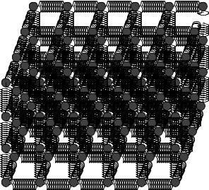
Figure 127: An idealized simple cubic lattice of atoms separated by the “springs” of interatomic forces that hold them in equilibrium positions. The equilibrium separation of the atoms as a.

As usual, we will deal with all of this complexity by ignoring most of it for now and considering an “ideal” case where a single kind of atoms lined up in a regular simple cubic lattice is su cient to help us understand properties that will hold, with di erent values of course, even for amorphous or structured solids. This is illustrated in figure 127, which is basically a mental cartoon model for a generic solid – lots of atoms in a regular cubic lattice with a cube side a, where the interactomic

Finally, we rearrange this by putting all of the extra terms together as follows:

to be Young’s Modulus. With these definitions, the equation above states that:

Compressive or extensive Stress applied to a solid equals Young’s Modulus times the Strain.

Note well that we can rearrange this equation into “Hooke’s Law” as follows:

which basically states that any given chunk of material behaves like a spring when forces are applied to stretch or compress it, with a spring constant K that is proportional to the cross sectional area A and inversely proportional to the length L! Young’s modulus is the material-dependent contribution from the actual geometry and interaction potential energy that holds the material together, but the rest of the dependence is generic, and applies to all materials.

This scaling behavior of the response of solid (or liquid, or gaseous) matter to applied forces is the important take-home conceptual lesson of this section. Substances like bone or steel or wood or nearly anything are stronger – respond less to an applied force – as they get thicker, and are weaker – respond more to an applied force – as they get longer. This intuitive understanding can be made quantitatively precise to be sure (and for e.g. engineers or orthopedic surgeons will have to be quantitatively precise as they craft buildings that won’t fall down or artificial hips or bones that mimic natural ones) but is su cient in and of itself for people to see the world through new eyes, to understand why there are building codes for houses and decks governing the lengths and cross-sectional areas of support beams and joists and so on. We’ll explore a few of these applications later, but first let us relatively quickly extend the linear extension/compression result to sideways forces and understand shear.

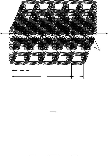
9.5.4: Shear Forces and the Shear Modulus

If we imagine taking our chunk of model solid pictured in figure 127 above and pushing sideways on the top to the right while the bottom is locked to a table by e.g. static friction on the bottom, we are applying a shear force – one that bends the material sideways instead of stretching or compressing it. The layers of the material all shift sideways by an amount that distributes the shear force between all of the layers as shown and the material deforms at an angle θ as shown.

A fully microscopic derivation of the response is still quite possible, but not quite as simple as that for Young’s modulus above. For that reason we will content ourselves with a simple heuristic extension of the scaling ideas we learned in the previous section.

The displacement layer to layer required to oppose a given shear force is going to be inversely proportional to the thickness of the material L, because the longer the material is, the more layers there are to split the restoring force among. So we expect Fs to be proportional to 1/L. The work we do as the material bends comes primarily from the stretching of the vertical bonds. The number of vertical bonds is proportional to the cross-sectional area A of the material at the shear surface on the top and bottom. More bonds, a stronger force for a given displacement. We expect Fs to

be proportional to A. As before, we expect the response to depend on the microscopic properties of the material and its structure in some way – we wrap all our ignorance of these properties into a modulus that we can more easily measure in the lab than compute from first principles. We then assemble these scaling results into:

where Ms is the shear modulus – the equivalent of Young’s modulus for shear forces. Once again

In words:

Shear Stress applied to a solid equals the Shear Modulus times the Strain.

where note well the minus sign that as always means that the reaction force opposes the applied shear force, trying to make x smaller in magnitude no matter what direction the material is being bent.

Shear stress is how springs really work! A “spring” is just a very long piece of material wrapped around into a coil so that when the ends are pulled, it produces shear stress spread out across the entire coil! So it is not an accident that we discover Hooke’s Law buried within this result – this is a (slighly handwaving) microscopic derivation of Hooke’s Law:

From this, we can predict how the strength of springs will vary according to the length of the wire in the coil L and its thickness A. Pretty cool!

9.5.5: Deformation and Fracture

What happens when one stretches or compresses or shears a material by an amount (per bond) that is not small? Here is a verbal description of what we might expect based on the microscopic model above and our own experience.

For a range of (relatively small) stresses, the strain remains a linear response – proportional to the stress, acting in a direction opposed to the stress. As one increases the stress, then, the first thing that happens is that the response becomes non-linear. Each additional increment of stress produces more than a linear increment of strain stretching, and quite possible less than a linear increment compressing, as one can understand from the graph of a typical interatomic or intermolecular force above. Materials tend to resist compression better than extension because one can pull bonded atoms apart but one cannot cause two bonded atoms to interpenetrate with any reasonable force – they are very strongly repulsive when their electron clouds start to overlap but only weakly attractive as the electron clouds are pulled apart.

At some point, one adds enough energy to the bonds (doing work as one e.g. stretches the material) that atoms or molecules start to dislocate – leave their normal place in the lattice or structure and migrate someplace else. This leaves behind a defect – a missing atom or molecule in the structure – and correspondingly weakens the entire structure. This migration tends to be permanent – even if one releases the stress on the material, it does not return to its original state but

remains stretched, compressed, or bent out of place. This region is one of permanent deformation of the material, as when one bends a paper clip.

Finally, if one continues to ratchet up the stress, at some point the number of defects introduced reaches a critical point and each new defect produced weakens the material enough that another defect is produced without further increase in stress, as the number of bonds over which the stress is distributed decreases with each new defect. The number of defects “explodes”, creating a fracture plane and the material breaks.

Figure 129: The slope of the linear response part of the curve is Young’s Modulus (note well the absolute magnitude signs). A marks the point where nonlinear response is first apparent. B marks the boundary where dislocations occur and permanent deformation of the material begins. C marks the point where there is a chain reaction – each defect produced produces on average at least one more defect at the same stress, so that the material “instantly” fractures.

These behaviors – and the critical points where the behavior changes – are summarized on the graph in figure 129.

Materials are not just characterized by their moduli. Moduli describe only the simple linear response regime. Furthermore, the moduli themselves depend on how far the atoms or molecules of the material are spending part of their time away from equilibrium without stress of any sort, because the material has a temperature (basically, a mechanical energy per atom that is larger than the minimum associated with sitting at the equilibrium point, at rest). In thermal equilibrium, each atom is already oscillating back and forth around its equilibrium position and temperature increases alone are su cient to drive the system through the same series of states – linear and nonlinear response where it can cool back to the original structure, nonlinear response that introduces defects so that the material “starts to melt” and doesn’t come back to its original state, followed by melting instead of fracture when the energy per bond no longer keeps atoms localized to a lattice or structure at all. When one mixes heating and stress, one can get many di erent ranges of physical behavior.

One last qualitative measure of interest is brittleness or toughness – a measure of how likely a material is to bend versus fracture when stresses are applied. Some materials, such as steel, are very tough and not very brittle – they do not easily deform or fracture. Others, like diamond, can be very hard indeed but are easy to fracture – they are brittle.

Human bone varies tremendously in the range of its brittleness with the lifetime of the human involved, with genetic factors, with dietary factors, and with the history of the person involved. Young people (on average) have bones that bend easily but aren’t very brittle. Old people have bones that become progressively more brittle as they decalcify with age or disease. Normal adults tend to fall in between – bones that are not as flexible but that are also not particularly brittle.