Week 10: The Wave Equation

a)Light string (medium) to heavy string (medium): Transmitted pulse right side up, reflected pulse inverted. (A fixed string boundary is the limit of attaching to an “infinitely heavy string”).

b)Heavy string to light string: Transmitted pulse right side up, reflected pulse right side up. (a free string boundary is the limit of attaching to a “massless string”).

10.1: Waves

We have seen how a particle on a spring that creates a restoring force proportional to its displacement from an equilibrium position oscillates harmonically in time about that equilibrium. What happens if there are many particles, all connected by tiny “springs” to one another in an extended way? This is a good metaphor for many, many physical systems. Particles in a solid, a liquid, or a gas both attract and repel one another with forces that maintain an average particle spacing. Extended objects under tension or pressure such as strings have components that can exert forces on one another. Even fields (as we shall learn next semester) can interact so that changes in one tiny element of space create changes in a neighboring element of space.

What we observe in all of these cases is that changes in any part of the medium ”propagate” to other parts of the medium in a very systematic way. The motion observed in this propagation is called a wave. We have all observed waves in our daily lives in many contexts. We have watched water waves propagate away from boats and raindrops. We listen to sound waves (music) generated by waves created on stretched strings or from tubes driven by air and transmitted invisibly through space by means of radio waves. We read these words by means of light, an electromagnetic wave. In advanced physics classes one learns that all matter is a sort of quantum wave, that indeed everything is really a manifestation of waves.

It therefore seems sensible to make a first pass at understanding waves and how they work in general, so that we can learn and understand more in future classes that go into detail.

The concept of a wave is simple – it is an extended structure that oscillates in both space and in time. We will study two kinds of waves at this point in the course:

•Transverse Waves (e.g. waves on a string). The displacement of particles in a transverse wave is perpendicular to the direction of the wave itself.

•Longitudinal Waves (e.g. sound waves). The displacement of particles in a longitudinal wave is in the same direction that the wave propagates in.

Some waves, for example water waves, are simultaneously longitudinal and transverse. Transverse waves are probably the most important waves to understand for the future; light is a transverse wave. We will therefore start by studying transverse waves in a simple context: waves on a stretched string.

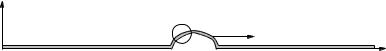
Figure 132: A uniform string is plucked or shaken so as to produce a wave pulse that travels at a speed v to the right. The circled region is examined in more detail in the next figure.

10.2: Waves on a String

Suppose we have a uniform stretchable string (such as a guitar string) that is pulled at the ends so that it is under tension T . The string is characterized by its mass per unit length µ – thick guitar strings have more mass per unit length than thin ones but little else. It is fairly harmless at this point to imagine that the string is fixed to pegs at the ends that maintain the tension. Our experience of such things leads us to expect that the stretched string will form an almost perfectly straight line unless we pluck it or otherwise bend some other shape upon it. We will impose coordinates upon this string such that x runs along its (undisplaced) equilibrium position and y describes the vertical displacement of any given bit of the string.

Now imagine that we have plucked the string somewhere between the end points so that it is displaced in the y-direction from its equilibrium (straight) stretched position and has some curved shape, as portrayed in figure 132. The tension T , recall, acts all along the string, but because the string is curved the force exerted on any small bit of string does not balance. This inspires us to try to write Newton’s Second Law not for the entire string itself, but for just a tiny bit of string, indeed a di erential bit of string.

We thus zoom in on just a small chunk of the string in the region where we have stretched or shaken a wave pulse as illustrated by the figure above. If we blow this small segment up, perhaps we can find a way to write the unbalanced forces out in a way we can deal with algebraically.

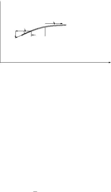
This is shown in figure 133, where I’ve indicated a short segment/chunk of the string of length x by cross-hatching it. We would like to write Newton’s 2nd law for that chunk. As you can see, the same magnitude of tension T pulls on both ends of the chunk, but the tension pulls in slightly

di erent directions, tangent to the string at the end points.

If θ is small, the components of the tension in the x-direction:

are nearly equal and in opposite directions and hence nearly perfectly cancel (where we have used the small angle approximation to the Taylor series for cosine:

for small θ 1).

Each bit of string therefore moves more or less straight up and down, and a useful solution is described by y(x, t), the y displacement of the string at position x and time t. The permitted solutions must be continuous if the string does not break. It is worth noting that not all waves involving moving up and down only – this initial example is called a transverse wave, but other kinds of waves exist. Sound waves, for example, are longitudinal compression waves, with the motion back and forth along the direction of motion and not at right angles to it. Surface waves on water are a mixture, they involve the water both moving up and down and back and forth. But for the moment we’ll stick with these very simple transverse waves on a string because they already exhibit most of the properties of far more general waves you might learn more about later on.

y

θ2 T θ1

x

T

x

Figure 133: The forces exerted on a small chunk of the string by the tension T in the string. Note that we neglect gravity in this treatment, assuming that it is much too small to bend the stretched string significantly (as is indeed the case, for a taut guitar string).

In the y-direction, we find write the force law by considering the total y-components of the sum of the force exerted by the tension on the ends of the chunk:

The quantity Tµ has to have units of Lt22 which is a velocity squared.

We therefore formulate this as the one dimensional wave equation:

are the velocity(s) of the wave on the string. This is a second order linear homogeneous di erential equation and has (as one might imagine) well known and well understood solutions.

Note well: At the tension in the string increases, so does the wave velocity. As the mass density of the string increases, the wave velocity decreases. This makes physical sense. As tension goes up the restoring force is greater. As mass density goes up one accelerates less for a given tension.