Добавил:
Upload Опубликованный материал нарушает ваши авторские права? Сообщите нам.
Вуз: Предмет: Файл:
intro_physics_1.pdf
Скачиваний:
52
Добавлен:
08.02.2016
Размер:
5.79 Mб
Скачать

346

Week 8: Fluids

Below a critical speed, the dynamic flow of a moving fluid tends to be laminar, where every bit of fluid moves parallel to its neighbors in response to pressure di erentials and around obstacles. Above that speed it becomes turbulent flow. Turbulent flow is quite di cult to treat mathematically and is hence beyond the scope of this introductory course – we will restrict our attention to ideal fluids either static or in laminar flow.

We will now use these general properties and definitions, plus our existing knowledge of physics, to deduce a number of important properties of and laws pertaining to static fluids, fluids that are in static equilibrium.

Static Fluids

8.1.6: Pressure and Confinement of Static Fluids

A

Fleft Fright

Fluid (density ρ)

V

Confining box

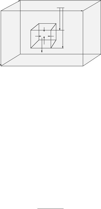
Figure 102: A fluid in static equilibrium confined to a sealed rectilinear box in zero gravity.

In figure 102 we see a box of a fluid that is confined within the box by the rigid walls of the box. We will imagine that this particular box is in “free space” far from any gravitational attractor and is therefore at rest with no external forces acting on it. We know from our intuition based on things like cups of co ee that no matter how this fluid is initially stirred up and moving within the container, after a very long time the fluid will damp down any initial motion by interacting with the walls of the container and arrive at static equilibrium133.

A fluid in static equilibrium has the property that every single tiny chunk of volume in the fluid has to independently be in force equilibrium – the total force acting on the di erential volume chunk must be zero. In addition the net torques acting on all of these di erential subvolumes must be zero, and the fluid must be at rest, neither translating nor rotating. Fluid rotation is more complex than the rotation of a static object because a fluid can be internally rotating even if all of the fluid in the outermost layer is in contact with a contain and is stationary. It can also be turbulent – there can be lots of internal eddies and swirls of motion, including some that can exist at very small length scales and persist for fair amounts of time. We will idealize all of this – when we discuss static properties of fluids we will assume that all of this sort of internal motion has disappeared.

We can now make a few very simple observations about the forces exerted by the walls of the container on the fluid within. First of all the mass of the fluid in the box above is clearly:

M = ρ V

(703)

133This state will also entail thermodynamic equilibrium with the box (which must be at a uniform temperature) and hence the fluid in this particular non-accelerating box has a uniform density.

Week 8: Fluids

347

where V is the volume of the box. Since it is at rest and remains at rest, the net external force exerted on it (only) by the the box must be zero (see Week 4). We drew a symmetric box to make it easy to see that the magnitudes of the forces exerted by opposing walls are equal Fleft = Fright (for example). Similarly the forces exerted by the top and bottom surfaces, and the front and back surfaces, must cancel.

The average velocity of the molecules in the box must be zero, but the molecules themselves will generally not be at rest at any nonzero temperature. They will be in a state of constant motion where they bounce elastically o of the walls of the box, both giving and receiving an impulse (change in momentum) from the walls as they do. The walls of any box large enough to contain many molecules thus exerts a nearly continuous nonzero force that confines any fluid not at zero temperature134.

From this physical picture we can also deduce an important scaling property of the force exerted by the walls. We have deliberately omitted giving any actual dimensions to our box in figure 102. Suppose (as shown) the cross-sectional area of the left and right walls are A originally. Consider now what we expect if we double the size of the box and at the same time add enough additional fluid for the fluid density to remain the same, making the side walls have the area 2ΔA. With twice the area (and twice the volume and twice as much fluid), we have twice as many molecular collisions per unit time on the doubled wall areas (with the same average impulse per collision). The average force exerted by the doubled wall areas therefore also doubles.

From this simple argument we can conclude that the average force exerted by any wall is proportional to the area of the wall. This force is therefore most naturally expressible in terms of pressure, for example:

Fleft = Pleft A = Pright A = Fright

(704)

which implies that the pressure at the left and right confining walls is the same:

Pleft = Pright = P

(705)

, and that this pressure describes the force exerted by the fluid on the walls and vice versa. Again, the exact same thing is true for the other four sides.

There is nothing special about our particular choice of left and right. If we had originally drawn a cubic box (as indeed we did) we can easily see that the pressure P on all the faces of the cube must be the same and indeed (as we shall see more explicitly below) the pressure everywhere in the fluid must be the same!

That’s quite a lot of mileage to get out of symmetry and the definition of static equilibrium, but there is one more important piece to get. This last bit involves forces exerted by the wall parallel to its surface. On average, there cannot be any! To see why, suppose that one surface, say the left one, exerted a force tangent to the surface itself on the fluid in contact with that surface. An important property of fluids is that one part of a fluid can move independent of another so the fluid in at least some layer with a finite thickness near the wall would therefore experience a net force and would accelerate. But this violates our assumption of static equilibrium, so a fluid in static equilibrium exerts no tangential force on the walls of a confining container and vice versa.

We therefore conclude that the direction of the force exerted by a confining surface with an area A on the fluid that is in contact with it is:

~

(706)

F = P Anˆ

where nˆ is an inward-directed unit vector perpendicular to (normal to) the surface. This final rule permits us to handle the force exerted on fluids confined to irregular amoebic blob shaped containers, or balloons, or bags, or – well, us, by our skins and vascular system.

134Or at a temperature low enough for the fluid to freeze and becomes a solid

348

Week 8: Fluids

Note well that this says nothing about the tangential force exerted by fluids in relative motion to the walls of the confining container. We already know that a fluid moving across a solid surface will exert a drag force, and later this week we’ll attempt to at least approximately quantify this.

Next, let’s consider what happens when we bring this box of fluid135 down to Earth and consider what happens to the pressure in a box in near-Earth gravity.

8.1.7: Pressure and Confinement of Static Fluids in Gravity

The principle change brought about by setting our box of fluid down on the ground in a gravitational field (or equivalently, accelerating the box of fluid uniformly in some direction to develop a pseudo- gravitational field in the non-inertial frame of the box) is that an additional external force comes into play: The weight of the fluid. A static fluid, confined in some way in a gravitational field, must support the weight of its many component parts internally, and of course the box itself must support the weight of the entire mass M of the fluid.

As hopefully you can see if you carefully read the previous section. The only force available to provide the necessary internal support or confinement force is the variation of pressure within the fluid. We would like to know how the pressure varies as we move up or down in a static fluid so that it supports its own weight.

There are countless reasons that this knowledge is valuable. It is this pressure variation that hurts your ears if you dive deep into the water or collapses submarines if they dive too far. It is this pressure variation that causes your ears to pop as you ride in a car up the side of a mountain or your blood to boil into the vacuum of space if you ride in a rocket all the way out of the atmosphere without a special suit or vehicle that provides a personally pressurized environment. It is this pressure variation that will one day very likely cause you to have varicose veins and edema in your lower extremities from standing on your feet all day – and can help treat/reverse both if you stand in 1.5 meter deep water instead of air. The pressure variation drives water out of the pipes in your home when you open the tap, helps lift a balloon filled with helium, floats a boat but fails to float a rock.

We need to understand all of this, whether our eventual goal is to become a physicist, a physician, an engineer, or just a scientifically literate human being. Let’s get to it.

Here’s the general idea. If we consider a tiny (eventually di erentially small) chunk of fluid in force equilibrium, gravity will pull it down and the only thing that can push it up is a pressure di erence between the top and the bottom of the chunk. By requiring that the force exerted by the pressure di erence balance the weight, we will learn how the pressure varies with increasing depth.

For incompressible fluids, this is really all there is to it – it takes only a few lines to derive a lovely formula for the increase in pressure as a function of depth in an incompressible liquid.

For gases there is, alas, a small complication. Compressible fluids have densities that increase as the pressure increases. This means that boxes of the same size also have more mass in them as one descends. More mass means that the pressure di erence has to increase, faster, which makes the density/mass greater still, and one discovers (in the end) that the pressure varies exponentially with depth. Hence the air pressure drops relatively quickly as one goes up from the Earth’s surface to very close to zero at a height of ten miles, but the atmosphere itself extends for a very long way into space, never quite dropping to “zero” even when one is twenty or a hundred miles high.

As it happens, the calculus for the two kinds of fluids is the same up to a given (very important) common point, and then di ers, becoming very simple indeed for incompressible fluids and a bit more di cult for compressible ones. Simple solutions su ce to help us build our conceptual understanding; we will therefore treat incompressible fluids first and everybody is responsible for understanding

135It’s just a box of rain. I don’t know who put it there...

Week 8: Fluids

349

them. Physics majors, math majors, engineers, and people who love a good bit of calculus now and then should probably continue on and learn how to integrate the simple model provided for compressible fluids.

x


P(0) =

P0

0


y


y

z


x

Ft


P(z)


F


Fr


l


z


z + z


Fb


P(z +

z)


mg


Fluid (density ρ)

z

Figure 103: A fluid in static equilibrium confined to a sealed rectilinear box in a near-Earth gravitational field ~g. Note well the small chunk of fluid with dimensions x, y, z in the middle of the fluid. Also note that the coordinate system selected has z increasing from the top of the box down, so that z can be thought of as the depth of the fluid.

In figure 103 a (portion of) a fluid confined to a box is illustrated. The box could be a completely sealed one with rigid walls on all sides, or it could be something like a cup or bucket that is open on the top but where the fluid is still confined there by e.g. atmospheric pressure.

Let us consider a small (eventually infinitesimal) chunk of fluid somewhere in the middle of the container. As shown, it has physical dimensions x, y, z; its upper surface is a distance z below the origin (where z increases down and hence can represent “depth”) and its lower surface is at depth z + z. The areas of the top and bottom surfaces of this small chunk are e.g. Atb = x y, the areas of the sides are x z and y z respectively, and the volume of this small chunk is

V = x y z.

This small chunk is itself in static equilibrium – therefore the forces between any pair of its horizontal sides (in the x or y direction) must cancel. As before (for the box in space) Fl = Fr in magnitude (and opposite in their y-direction) and similarly for the force on the front and back faces in the x-direction, which will always be true if the pressure does not vary horizontally with variations in x or y. In the z-direction, however, force equilibrium requires that:

Ft + mg − Fb = 0

(707)

(where recall, down is positive).


The only possible source of Ft and Fb are the pressure in the fluid itself

which will vary

with the depth z: Ft = P (zAtb and Fb = P (z + zAtb. Also, the mass of fluid in the (small)

box is m = ρ

V (using our ritual incantation “the mass of the chunks is...”). We can thus write:


P (zx y + ρx y

z)g − P (z +

zx y = 0

(708)

or (dividing by

x y z and rearranging):


P

=

P (z +

z) − P (z)

= ρg

(709)


z


z