6.7: Precession of a Top

important problem to clearly and quantitatively understand even in this introductory course because it is the basis of Magnetic Resonance Imaging (MRI) in medicine, the basis of understanding quantum phenomena ranging from spin resonance to resonant emission from two-level atoms for physicists, and the basis for gyroscopes to the engineer. Evvybody need to know it, in other words, no fair hiding behind the sputtered “but I don’t need to know this crap” weasel-squirm all too often uttered by frustrated students.

Look, I’ll bribe you. This is one of those topics/problems that I guarantee will be on at least one quiz, hour exam, or the final this semester. That is, mastering it will be worth at least ten points of your total credit, and in most years it is more likely to be thirty or even fifty points. It’s that important! If you master it now, then understanding the precession of a proton around a magnetic field will be a breeze next semester. Otherwise, you risk the additional 10-50 points it might be worth next semester.

If you are a sensible person, then, you will recognize that I’ve just made it worth your while to invest the time required to completely understand precession in terms of vector torque, and to be able to derive the angular frequency of precession, ωp – which is our goal. I’ll show you three ways to do it, don’t worry, and any of the three will be acceptable (although I prefer that you use the second or third as the first is a bit too simple, it gets the right answer but doesn’t give you a good feel for what happens if the forces that produce the torque change in time).

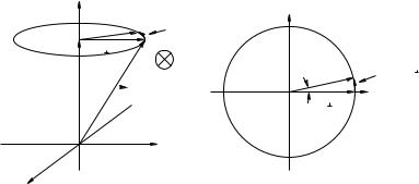
First, though, let’s understand the phenonenon. If figure ?? above, a simple top is shown spinning at some angular velocity ω (not to be confused with ωp, the precession frequency). We will idealize this particular top as a massive disk with mass M , radius R, spinning around a rigid massless spindle that is resting on the ground, tipped at an angle θ with respect to the vertical.

We begin by noting that this top is symmetric, so we can easily compute the magnitude and direction of its angular momentum:

Using the “grasp the axis” version of the right hand rule, we see that in the example portrayed this angular momentum points in the direction from the pivot at the point of contact between the spindle and the ground and the center of mass of the disk along the axis of rotation.

Second, we note that there is a net torque exerted on the top relative to this spindle-ground contact point pivot due to gravity. There is no torque, of course, from the normal force that holds up the top, and we are assuming the spindle and ground are frictionless. This torque is a vector :

into the page as drawn above, where z is vertical.

Third we note that the torque will change the angular momentum by displacing it into the page

~

in the direction of the torque. But as it does so, the plane containing the D and M gzˆ will be rotated a tiny bit around the z (precession) axis, and the torque will also shift its direction to

~

remain perpendicular to this plane. It will shift L a bit more, which shifts ~τ a bit more and so on.

~

In the end L will precess around z, with ~τ precessing as well, always π/2 ahead .

exactly like the cone swept out in the unbalanced rotation problems above and we can use similar considerations to relate the magnitude of the torque (known above) to the change of angular momentum per period. This is the simplest (and least accurate) way to find the precession frequency. Let’s start by giving this a try:

x

“overhead view” of the trajectory of L , the component of L perpendicular to the z-axis.

~

discussion of the kinematics of circular motion – L sweeps out a cone around the z-axis where Lz and the magnitude of L remain constant.

as before. Note well that because this time we could take the limit as t → 0, we get an expression that is good at any instant in time, even if the top is in a rocket ship (an accelerating frame) and g → g′ is varying in time!

This still isn’t the most elegant approach. The best approach, although it does use some real calculus, is to just write down the equation of motion for the system as di erential equations and

~

solve them for both L(t) and for ωp.

Example 6.7.3: Finding ωp from Calculus

Way back at the beginning of this section we wrote down Newton’s Second Law for the rotation of the gyroscope directly:

If we di erentiate the first expression and substitute the second into the first (and vice versa) we transform this pair of coupled first order di erential equations for Lx and Ly into the following pair of second order di erential equations:

These (either one) we will learn to recognize as the di erential equation of motion for the simple harmonic oscillator. A particular solution of interest (that satisfies the first order equations above) might be:

~

which is then the exact solution to the equation of motion for L(t) that describes the actual cone being swept out, with no hand-waving or limit taking required.

The only catch to this approach is, of course, that we don’t know how to solve the equation of motion yet, and the very phrase “second order di erential equation” strikes terror into our hearts in spite of the fact that we’ve been solving one after another since week 1 in this class! All of the equations of motion we have solved from Newton’s Second Law have been second order ones, after all – it is just that the ones for constant acceleration were directly integrable where this set is not, at least not easily.

It is pretty easy to solve for all of that, but we will postpone the actual solution until later. In the meantime, remember, you must know how to reproduce one of the three derivations above for ωp, the angular precession frequency, for at least one quiz, test, or hour exam. Not to mention a homework problem, below. Be sure that you master this because precession is important.

One last suggestion before we move on to treat angular collisions. Most students have a lot of experience with pushes and pulls, and so far it has been pretty easy to come up with everyday experiences of force, energy, one dimensional torque and rolling, circular motion, and all that. It’s not so easy to come up with everyday experiences involving vector torque and precession. Yes, may of you played with tops when you were kids, yes, nearly everybody rode bicycles and balancing and steering a bike involves torque, but you haven’t really felt it knowing what was going on.

The only device likely to help you to personally experience torque “with your own two hands” is the bicycle wheel with handles and the string that was demonstrated in class. I urge you to take a turn spinning this wheel and trying to turn it by means of its handles while it is spinning, to spin it and suspend it by the rope attached to one handle and watch it precess. Get to where you can predict the direction of precession given the direction of the spin and the handle the rope is attached to, get so you have experience of pulling it (say) in and out and feeling the handles deflect up and down or vice versa. Only thus can you feel the nasty old cross product in both the torque and the angular momentum, and only thus can you come to understand torque with your gut as well as your head.