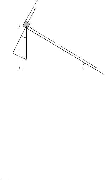
y

N

m

θ

mg

L

H

θ

x

Figure 11: A good choice of coordinate frame has (say) the x-coordinate lined up with the total force and hence direction of motion.

From this point on the solution should be familiar – since vy (0) = 0 and y(0) = 0, y(t) = 0 and we can ignore y altogether and the problem is now one dimensional! See if you can find how long it takes for the block to reach bottom, and how fast it is going when it gets there. You should find that vbottom = √2gH, a familiar result (see the very first example of the dropped ball) that suggests that there is more to learn, that gravity is somehow “special” if a ball can be dropped or slide down from a height H and reach the bottom going at the same speed either way!

1.9: Circular Motion

So far, we’ve solved only two dimensional problems that involved a constant acceleration in some specific direction. Another very general (and important!) class of motion is circular motion. This could be: a ball being whirled around on a string, a car rounding a circular curve, a roller coaster looping-the-loop, a bicycle wheel going round and round, almost anything rotating about a fixed axis has all of the little chunks of mass that make it up going in circles!

Circular motion, as we shall see, is “special” because the acceleration of a particle moving in a circle towards the center of the circle has a value that is completely determined by the geometry of this motion. The form of centripetal acceleration we are about to develop is thus a kinematic relation – not dynamical. It doesn’t matter which force(s) or force rule(s) o of the list above make something actually move around in a circle, the relation is true for all of them. Let’s try to understand this.

v

v

r

Figure 12: A way to visualize the motion of a particle, e.g. a small ball, moving in a circle of radius r. We are looking down from above the circle of motion at a particle moving counterclockwise around the circle. At the moment, at least, the particle is moving at a constant speed v (so that its velocity is always tangent to the circle.

1.9.1: Tangential Velocity

First, we have to visualize the motion clearly. Figure 12 allows us to see and think about the motion of a particle moving in a circle of radius r (at a constant speed, although later we can relax this to instantaneous speed) by visualizing its position at two successive times. The first position (where the particle is solid/shaded) we can imagine as occurring at time t. The second position (empty/dashed) might be the position of the particle a short time later at (say) t + t.

During this time, the particle travels a short distance around the arc of the circle. Because the length of a circular arc is the radius times the angle subtended by the arc we can see that:

Note Well! In this and all similar equations θ must be measured in radians, never degrees. In fact, angles measured in degrees are fundamentally meaningless, as degrees are an arbitrary partitioning of the circle. Also note that radians (or degrees, for that matter) are dimensionless – they are the ratio between the length of an arc and the radius of the arc (think 2π is the ratio of the circumference of a circle to its radius, for example).

The average speed v of the particle is thus this distance divided by the time it took to move it:

Of course, we really don’t want to use average speed (at least for very long) because the speed might be varying, so we take the limit that t → 0 and turn everything into derivatives, but it is much

This speed is directed tangent to the circle of motion (as one can see in the figure) and we will often refer to it as the tangential velocity. Sometimes I’ll even put a little “t” subscript on it to emphasize the point, as in:

but since the velocity is always tangent to the trajectory (which just happens to be circular in this case) we don’t really need it.

In this equation, we see that the speed of the particle at any instant is the radius times the rate that the angle is being swept out by by the particle per unit time. This latter quantity is a very, very useful one for describing circular motion, or rotating systems in general. We define it to be the angular velocity:

are both extremely useful expressions describing the kinematics of circular motion.

1.9.2: Centripetal Acceleration

v = vΔθ

v

Δθ

Figure 13: The velocity of the particle at t and t + t. Note that over a very short time t the speed of the particle is at least approximately constant, but its direction varies because it always has to be perpendicular to ~r, the vector from the center of the circle to the particle. The velocity swings through the same angle θ that the particle itself swings through in this (short) time.

Next, we need to think about the velocity of the particle (not just its speed, note well, we have to think about direction). In figure 13 you can see the velocities from figure 12 at time t and t + t placed so that they begin at a common origin (remember, you can move a vector anywhere you like as long as the magnitude and direction are preserved).

The velocity is perpendicular to the vector ~r from the origin to the particle at any instant of time. As the particle rotates through an angle θ, the velocity of the particle also must rotate through the angle θ while its magnitude remains (approximately) the same.

In time t, then, the magnitude of the change in the velocity is:

Consequently, the average magnitude of the acceleration is:

As before, we are interested in the instantaneous value of the acceleration, and we’d also like to determine its direction as it is a vector quantity. We therefore take the limit t → 0 and inspect the figure above to note that the direction in that limit is to the left, that is to say in the negative ~r direction! (You’ll need to look at both figures, the one representing position and the

other representing the velocity, in order to be able to see and understand this.) The instantaneous magnitude of the acceleration is thus:

where we have substituted equation 122 for ω (with a bit of algebra) to get the last couple of equivalent forms. The direction of this vector is towards the center of the circle.

The word “centripetal” means “towards the center”, so we call this kinematic acceleration the centripetal acceleration of a particle moving in a circle and will often label it:

A second way you might see this written or referred to is as the r-component of a vector in plane polar coordinates. In that case “towards the center” is in the −rˆ direction and we could write:

In most actual problems, though, it is easiest to just compute the magnitude ac and then assign the direction in terms of the particular coordinate frame you have chosen for the problem, which might well make “towards the center” be the positive x direction or something else entirely in your figure at the instant drawn.

This is an enormously useful result. Note well that it is a kinematic result – math with units

– not a dynamic result. That is, I’ve made no reference whatsoever to forces in the derivations above; the result is a pure mathematical consequence of motion in a 2 dimensional plane circle, quite independent of the particular forces that cause that motion. The way to think of it is as follows:

If a particle is moving in a circle at instantaneous speed v, then its acceleration towards the center of that circle is v2/r (or rω2 if that is easier to use in a given problem).

This specifies the acceleration in the component of Newton’s Second Law that points towards the center of the circle of motion! No matter what forces act on the particle, if it moves in a circle the component of the total force acting on it towards the center of the circle must be mac = mv2/r. If the particle is moving in a circle, then the centripetal component of the total force must have this value, but this quantity isn’t itself a force law or rule! There is no such thing as a “centripetal force”, although there are many forces that can cause a centripetal acceleration in a particle moving in circular trajectory.

Let me say it again, with emphasis: A common mistake made by students is to confuse mv2/r with a “force rule” or “law of nature”. It is nothing of the sort. No special/new force “appears” because of circular motion, the circular motion is caused by the usual forces we list above in some combination that add up to mac = mv2/r in the appropriate direction. Don’t make this mistake one a homework problem, quiz or exam! Think about this a bit and discuss it with your instructor if it isn’t completely clear.

Example 1.9.1: Ball on a String

At the bottom of the trajectory, the tension T in the string points straight up and the force mg points straight down. No other forces act, so we should choose coordinates such that one axis lines up with these two forces. Let’s use +y vertically up, aligned with the string. Then: