9.3: Damped Oscillation

k

Damping fluid (b)

m

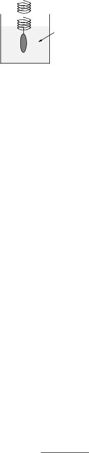
Figure 121: A smooth convex mass on a spring that is immersed in a suitable damping liquid experiences a linear damping force due to viscous interaction with the fluid in laminar flow. This idealizes the forces to where we can solve them and understand semi-quantitatively how to describe damped oscillation.

We’ll pick the simplest possible one, illustrated in figure 121 above – a linear damping force such as we would expect to observe in laminar flow around the oscillating object as long as it moves at speeds too low to excite turbulence in the surrounding fluid.

As before (see e.g. week 2) b is called the damping constant or damping coe cient. With this form we can get an exact solution to the di erential equation easily (good), get a preview of a solution we’ll need next semester to study LRC circuits (better), and get a very nice qualitative picture of damping even when the damping force is not precisely linear (best).

As before, we write Newton’s Second Law for a mass m on a spring with spring constant k and a damping force −bv:

which is the “standard form” for a damped mass on a spring and (within fairly obvious substitutions) for the general linearly damped SHO.

This is still a linear, second order, homogeneous, ordinary di erential equation, but now we cannot just guess x(t) = A cos(ωt) because the first derivative of a cosine is a sine! This time we really must guess that x(t) is a function that is proportional to its own first derivative!

We therefore guess x(t) = Aeαt as before, substitute for x(t) and its derivatives, and get:

As before, we exclude the trivial solution x(t) = 0 as being too boring to solve for (requiring that A =6 0, that is) and are left with the characteristic equation for α:

This quadratic equation must be satisfied in order for our guess to be a nontrivial solution to the damped SHO ODE.

To solve for α we have to use the dread quadratic formula:

This isn’t quite where we want it. We expect from experience and intuition that for weak damping we should get an oscillating solution, indeed one that (in the limit that b → 0) turns back into our familiar solution to the undamped SHO above. In order to get an oscillating solution, the argument of the square root must be negative so that our solution becomes a complex exponential solution as before!

This motivates us to factor a −4k/m out from under the radical (where it becomes iω0, where p

ω0 = k/m is the frequency of the undamped oscillator with the same mass and spring constant). In addition, we simplify the first term and get:

As was the case for the undamped SHO, there are two solutions:

This, you will note, is not terribly simple or easy to remember! Yet you are responsible for knowing it. You have the usual choice – work very hard to memorize it, or learn to do the derivation(s).

I personally do not remember it at all save for a week or two around the time I teach it each semester. Too big of a pain, too easy to derive if I need it. But here you must suit yourself – either memorize it the same way that you’d memorize the digits of π, by lots and lots of mindless practice, or learn how to solve the equation, as you prefer.

Without recapitulating the entire argument, it should be fairly obvious that can take the real part of their sum, get formally identical terms, and combine them to get the general real solution:

where A is the real initial amplitude and φ determines the relative phase of the oscillator. The only two di erences, then, are that the frequency of the oscillator is shifted to ω′ and the whole solution is exponentially damped in time.

9.3.1: Properties of the Damped Oscillator

There are several properties of the damped oscillator that are important to know.

•The amplitude damps exponentially as time advances. After a certain amount of time, the amplitude is halved. After the same amount of time, it is halved again.

•The frequency ω′ is shifted so that it is smaller than ω0, the frequency of the identical but undamped oscillator with the same mass and spring constant.

•The oscillator can be (under)damped, critically damped, or overdamped. These terms are defined below.

•For exponential decay problems, recall that it is often convenient to define the exponential decay time, in this case:

This is the time required for the amplitude to go down to 1/e of its value from any starting time. For the purpose of drawing plots, you can imagine e = 2.718281828 ≈ 3 so that 1/e ≈ 1/3. Pay attention to how the damping time scales with m and b. This will help you develop a conceptual understanding of damping.

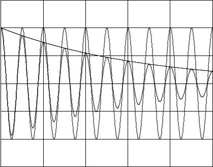
Figure 122: Two identical oscillators, one undamped (with ω0 = 2π, or if you prefer with an undamped period T0 = 1) and one weakly damped (b/m = 0.3).

Several of these properties are illustrated in figure 122. In this figure the exponential envelope of the damping is illustrated – this envelope determines the maximum amplitude of the oscillation as the total energy of the oscillating mass decays, turned into heat in the damping fluid. The period T ′ is indeed longer, but even for this relatively rapid damping, it is still nearly identical to T0! See if you can determine what ω′ is in terms of ω0 numerically given that ω0 = 2π and b/m = 0.3. Pretty close, right?

This oscillator is underdamped. An oscillator is underdamped if ω′ is real, which will be true

if:

An underdamped oscillator will exhibit true oscillations, eventually (exponentially) approaching zero amplitude due to damping.

The oscillator will then not oscillate – it will go to zero exponentially in the shortest possible time. This (and barely underdamped and overdamped oscillators) is illustrated in figure 123.

The oscillator is overdamped if ω′ is imaginary, which will be true if

In this case α is entirely real and has a component that damps very slowly. The amplitude goes to zero exponentially as before, but over a longer (possibly much longer) time and does not oscillate