Worse, the train is riding on the Earth, which is not exactly at rest relative to the sun, so we could describe the velocity of the block by adding the velocity of the Earth to that of the train and the block within the train. The kinetic energy in this case is so large that the di erence in the energy of the block due to its relative motion in the train coordinates is almost invisible against the huge energy it has in an inertial frame in which the sun is approximately at rest. Finally, as we discussed last week, the sun itself is moving relative to the galactic center or the “rest frame of the visible Universe”.

What, then, is the actual kinetic energy of the block?

I don’t know that there is such a thing. But the kinetic energy of the block in the inertial reference frame of any well-posed problem is 12 mv2, and that will have to be enough for us. As we will prove below, this definition makes the work done by the forces of nature consistent within the frame, so that our computations will give us answers consistent with experiment and experience in the frame coordinates.

3.2: The Work-Kinetic Energy Theorem

Let us now formally state the result we derived above using the new definitions of work and kinetic energy as the Work-Kinetic Energy Theorem (which I will often abbreviate, e.g. WKET) in one dimension in English:

The work done on a mass by the total force acting on it is equal to the change in its kinetic energy.

and as an equation that is correct for constant one dimensional forces only:

You will note that in the English statement of the theorem, I didn’t say anything about needing the force to be constant or one dimensional. I did this because those conditions aren’t necessary – I only used them to bootstrap and motivate a completely general result. Of course, now it is up to us to prove that the theorem is general and determine its correct and general algebraic form. We can, of course, guess that it is going to be the integral of this di erence expression turned into a di erential expression:

but actually deriving this for an explicitly non-constant force has several important conceptual lessons buried in the derivation. So much so that I’ll derive it in two completely di erent.

3.2.1: Derivation I: Rectangle Approximation Summation

First, let us consider a force that varies with position so that it can be mathematically described as a function of x, Fx(x). To compute the work done going between (say) x0 and some position xf that will ultimately equal the total change in the kinetic energy, we can try to chop the interval xf −x0 up into lots of small pieces, each of width x. x needs to be small enough that Fx basically doesn’t change much across it, so that we are justified in saying that it is “constant” across each interval, even though the value of the constant isn’t exactly the same from interval to interval. The

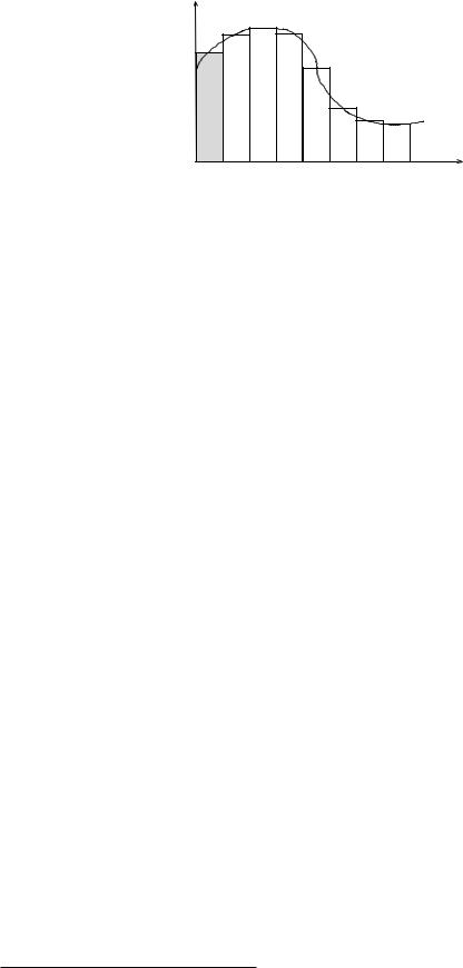
Figure 33: The work done by a variable force can be approximated arbitrarily accurately by summing Fx x using the average force as if it were a constant force across each of the “slices” of width x one can divide the entire interval into. In the limit that the width x → dx, this summation turns into the integral.

actual value we use as the constant in the interval isn’t terribly important – the easiest to use is the average value or value at the midpoint of the interval, but no matter what sensible value we use the error we make will vanish as we make x smaller and smaller.

In figure 33, you can see a very crude sketch of what one might get chopping the total interval x0 → xf up into eight pieces such that e.g. x1 = x0 + x, x2 = x1 + x,... and computing the work done across each sub-interval using the approximately constant value it has in the middle of the sub-interval. If we let F1 = Fx(x0 + x/2), then the work done in the first interval, for example, is F1 x, the shaded area in the first rectangle draw across the curve. Similarly we can find the work done for the second strip, where F2 = Fx(x1 + x/2) and so on. In each case the work done equals the change in kinetic energy as the particle moves across each interval from x0 to xf .

We then sum the constant acceleration Work-Kinetic-Energy theorem for all of these intervals:

where the internal changes in kinetic energy at the end of each interval but the first and last cancel. Finally, we let x go to zero in the usual way, and replace summation by integration. Thus:

lim

and we have generalized the theorem to include non-constant forces in one dimension82.

This approach is good in that it makes it very clear that the work done is the area under the curve Fx(x), but it buries the key idea – the elimination of time in Newton’s Second Law – way back in the derivation and relies uncomfortably on constant force/acceleration results. It is much more elegant to directly derive this result using straight up calculus, and honestly it is a lot easier, too.

82This is notationally a bit sloppy, as I’m not making it clear that as Deltax gets smaller, you have to systematically increase the number of pieces you divide xF − x0 into and so on, hoping that you all remember you intro calculus course and recognize this picture as being one of the first things you learned about integration...

3.2.2: Derivation II: Calculus-y (Chain Rule) Derivation

To do that, we simply take Newton’s Second Law and eliminate dt using the chain rule. The algebra is:

This is an elegant proof, one that makes it completely clear that time dependence is being eliminated in favor of the direct dependence of v on x. It is also clearly valid for very general one dimensional force functions; at no time did we assume anything about Fx other than its general integrability in the last step.

~

What happens if F is actually a vector force, not necessarily in acting only in one dimension? Well, the first proof above is clearly valid for Fx(x), Fy (y) and Fz (z) independently, so:

Z Z Z Z

~ ~

F · dℓ = Fxdx + Fy dy + Fz dz = Kx + Ky + Kz = K (254)

However, this doesn’t make the meaning of the integral on the left very clear.

x(t)

F

θ

F||

dL

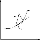
Figure 34: Consider the work done going along the particular trajectory ~x(t) where there is a force

~

F (~x) acting on it that varies along the way. As the particle moves across the small/di erential

~ ~

section dℓ, only the force component along dℓ does work. The other force component changes the direction of the velocity without changing its magnitude.

The best way to understand that is to examine a small piece of the path in two dimensions. In

~

figure 34 a small part of the trajectory of a particle is drawn. A small chunk of that trajectory dℓ represents the vector displacement of the object over a very short time under the action of the force

~

F acting there.

~ ~

The component of F perpendicular to dℓ doesn’t change the speed of the particle; it behaves like a centripetal force and alters the direction of the velocity without altering the speed. The component

~

parallel to dℓ, however, does alter the speed, that is, does work. The magnitude of the component

~

in this direction is (from the picture) F cos(θ) where θ is the angle between the direction of F and

~

the direction of dℓ.

That component acts (over this very short distance) like a one dimensional force in the direction of motion, so that

The next little chunk of ~x(t) has a di erent force and direction but the form of the work done and change in kinetic energy as the particle moves over that chunk is the same. As before, we can integrate from one end of the path to the other doing only the one dimensional integral of the path

~

element dℓ times F||, the component of F parallel to the path at that (each) point.

The vector operation that multiplies a vector by the component of another vector in the same

~

direction as the first is the dot (or scalar) product. The dot product between two vectors A and

~

B can be written more than one way (all equally valid):

The second form is connected to what we got above just adding up the independent cartesian component statements of the Work-Kinetic Energy Theorem in one (each) dimension, but it doesn’t help us understand how to do the integral between specific starting and ending coordinates along some trajectory. The first form of the dot product, however, corresponds to our picture:

Now we can see what the integral means. We have to sum this up along some specific path between ~x0 and ~x1 to find the total work done moving the particle along that path by the force. For di erential sized chunks, the “sum” becomes an integral and we integrate this along the path to get the correct statement of the Work-Kinetic Energy Theorem in 2 or 3 dimensions:

Note well that this integral may well be di erent for di erent paths connecting points ~x0 to ~x1! In the most general case, one cannot find the work done without knowing the path taken, because there are many ways to go between any two points and the forces could be very di erent along them.

Also, Note well: Energy is a scalar – just a number with a magnitude and units but no direction

– and hence is considerably easier to treat than vector quantities like forces.

In fact, force components perpendicular to the trajectory bend the trajectory with local curvature F = mv2/R but don’t speed the particle up or slow it down. This really simplifies problem solving, as we shall see.

We should think about using time-independent work and energy instead of time dependent Newtonian dynamics whenever the answer requested for a given problem is independent of time. The reason for this should now be clear: we derived the work-energy theorem (and energy conservation) from the elimination of t from the dynamical equations.

Let’s look at a few examples to see how work and energy can make our problem solving lives much better.

Example 3.2.1: Pulling a Block

Suppose we have a block of mass m being pulled by a string at a constant tension T at an angle θ with the horizontal along a rough table with coe cients of friction µs > µk. Typical questions