m

x

Figure 3: A mass m hangs on a spring with spring constant k. We would like to compute the amount x by which the string is stretched when the mass is at rest in static force equilibrium.

X

or (with x = x − x0, so that x is negative as shown)

Note that this result doesn’t depend on where the origin of the x-axis is, because x and x0 both change by the same amount as we move it around. In most cases, we will find the equilibrium position of a mass on a spring to be the most convenient place to put the origin, because then x and

x are the same!

In static equilibrium, ax = 0 (and hence, Fx = 0) and we can solve for x:

You will see this result appear in several problems and examples later on, so bear it in mind.

1.7: Simple Motion in One Dimension

Finally! All of that preliminary stu is done with. If you actually read and studied the chapter up to this point (many of you will not have done so, and you’ll be SORRReeee...) you should:

a)Know Newton’s Laws well enough to recite them on a quiz – yes, I usually just put a question like “What are Newton’s Laws” on quizzes just to see who can recite them perfectly, a really useful thing to be able to do given that we’re going to use them hundreds of times in the next 12 weeks of class, next semester, and beyond; and

b)Have at least started to commit the various force rules we’ll use this semester to memory.

I don’t generally encourage rote memorization in this class, but for a few things, usually very fundamental things, it can help. So if you haven’t done this, go spend a few minutes working on this before starting the next section.

All done? Well all rightie then, let’s see if we can actually use Newton’s Laws (usually Newton’s Second Law, our dynamical principle) and force rules to solve problems. We will start out very gently, trying to understand motion in one dimension (where we will not at first need multiple coordinate dimensions or systems or trig or much of the other stu that will complicate life later) and then, well, we’ll complicate life later and try to understand what happens in 2+ dimensions.

Here’s the basic structure of a physics problem. You are given a physical description of the problem. A mass m at rest is dropped from a height H above the ground at time t = 0; what happens to the mass as a function of time? From this description you must visualize what’s going on (sometimes but not always aided by a figure that has been drawn for you representing it in some way). You must select a coordinate system to use to describe what happens. You must write Newton’s Second Law in the coordinate system for all masses, being sure to include all forces or force rules that contribute to its motion. You must solve Newton’s Second Law to find the accelerations of all the masses (equations called the equations of motion of the system). You must solve the equations of motion to find the trajectories of the masses, their positions as a function of time, as well as their velocities as a function of time if desired. Finally, armed with these trajectories, you must answer all the questions the problem poses using algebra and reason and – rarely in this class

– arithmetic!

Simple enough.

Let’s put this simple solution methodology to the test by solving the following one dimensional, single mass example problem, and then see what we’ve learned.

Example 1.7.1: A Mass Falling from Height H

Let’s solve the problem we posed above, and as we do so develop a solution rubric – a recipe for solving all problems involving dynamics42! The problem, recall, was to drop a mass m from rest from a height H, algebraically find the trajectory (the position function that solves the equations of motion) and velocity (the time derivative of the trajectory), and then answer any questions that might be asked using a mix of algebra, intuition, experience and common sense. For this first problem we’ll postpone actually asking any question until we have these solutions so that we can see what kinds of questions one might reasonably ask and be able to answer.

The first step in solving this or any physics problem is to visualize what’s going on! Mass m? Height H? Drop? Start at rest? Fall? All of these things are input data that mean something when translated into algebraic ”physicsese”, the language of physics, but in the end we have to coordinatize the problem (choose a coordinate system in which to do the algebra and solve our equations for an answer) and to choose a good one we need to draw a representation of the problem.

Physics problems that you work and hand in that have no figure, no picture, not even additional hand-drawn decorations on a provided figure will rather soon lose points in the grading scheme! At first we (the course faculty) might just remind you and not take points o , but by your second assignment you’d better be adding some relevant artwork to every solution43. Figure 4 is what an

42At least for the next couple of weeks... but seriously, this rubric is useful all the way up to graduate physics.

43This has two benefits – one is that it actually is a critical step in solving the problem, the other is that drawing

engages the right hemisphere of your brain (the left hemisphere is the one that does the algebra). The right hemisphere is the one that controls formation of long term memory, and it can literally get bored, independently of the left hemisphere and interrupt your ability to work. If you’ve ever worked for a very long time on writing something very dry (left hemisphere) or doing lots of algebraic problems (left hemisphere) and found your eyes being almost irresistably drawn up to look out the window at the grass and trees and ponies and bright sun, then know that it is your “right brain” that has taken over your body because it is dying in there, bored out of its (your!) gourd.

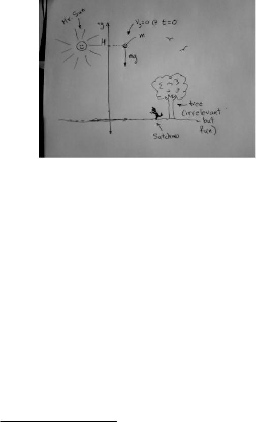
Figure 4: A picture of a ball being dropped from a height H, with a suitable one-dimensional coordinate system added. Note that the figure clearly indicates that it is the force of gravity that makes it fall. The pictures of Satchmo (my border collie) and the tree and sun and birds aren’t strictly necessary and might even be distracting, but my right brain was bored when I drew this picture and they do orient the drawing and make it more fun!

actual figure you might draw to accompany a problem might look like.

Note a couple of things about this figure. First of all, it is large – it took up 1/4+ of the unlined/white page I drew it on. This is actually good practice – do not draw postage-stamp sized figures! Draw them large enough that you can decorate them, not with Satchmo but with things like coordinates, forces, components of forces, initial data reminders. This is your brain we’re talking about here, because the paper is functioning as an extension of your brain when you use it to help solve the problem. Is your brain postage-stamp sized? Don’t worry about wasting paper – paper is cheap, physics educations are expensive. Use a whole page (or more) per problem solution at this point, not three problems per page with figures that require a magnifying glass to make out.

When I (or your instructor) solve problems with you, this is the kind of thing you’ll see us draw, over and over again, on the board, on paper at a table, wherever. In time, physicists become pretty good schematic artists and so should you. However, in a textbook we want things to be clearer and prettier, so I’ll redraw this in figure 5, this time with a computer drawing tool (xfig) that I’ll use for drawing most of the figures included in the textbook. Alas, it won’t have Satchmo, but it does have all of the important stu that should be on your hand-drawn figures.

Note that I drew two alternative ways of adding coordinates to the problem. The one on the left is appropriate if you visualize the problem from the ground, looking up like Satchmo, where the ground is at zero height. This might be e.g. dropping a ball o of the top of Duke Chapel, for example, with you on the ground watching it fall.

The one or the right works if you visualize the problem as something like dropping the same ball

To keep the right brain happy while you do left brained stu , give it something to do – listen to music, draw pictures or visualize a lot, take five minute right-brain-breaks and deliberately look at something visually pleasing. If your right brain is happy, you can work longer and better. If your right brain is engaged in solving the problem you will remember what you are working on much better, it will make more sense, and your attention won’t wander as much. Physics is a whole brain subject, and the more pathways you use while working on it, the easier it is to understand and remember!

Figure 5: The same figure and coordinate system, drawn “perfectly” with xfig, plus a second (alternative) coordinatization.

into a well, where the ground is still at “zero height” but now it falls down to a negative height H from zero instead of starting at H and falling to height zero. Or, you dropping the ball from the top of the Duke Chapel and counting “y = 0 as the height where you are up there (and the initial position in y of the ball), with the ground at y = −H below the final position of the ball after it falls.

Now pay attention, because this is important: Physics doesn’t care which coordinate system you use! Both of these coordinatizations of the problem are inertial reference frames. If you think about it, you will be able to see how to transform the answers obtained in one coordinate system into the corresponding answers in the other (basically subtract a constant H from the values of y in the left hand figure and you get y′ in the right hand figure, right?). Newton’s Laws will work perfectly in either inertial reference frame44, and truthfully there are an infinite number of coordinate frames you could choose that would all describe the same problem in the end. You can therefore choose the frame that makes the problem easiest to solve!

Personally, from experience I prefer the left hand frame – it makes the algebra a tiny bit prettier

– but the one on the right is really almost as good. I reject without thinking about it all of the frames where the mass m e.g. starts at the initial position yi = H/2 and falls down to the final position yf = −H/2. I do sometimes consider a frame like the one on the right with y positive pointing down, but it often bothers students to have “down” be positive (even though it is very natural to

~

orient our coordinates so that F points in the positive direction of one of them) so we’ll work into that gently. Finally, I did draw the x (horizontal) coordinate and ignored altogether for now the z coordinate that in principle is pointing out of the page in a right-handed coordinate frame. We don’t really need either of these because no aspect of the motion will change x or z (there are no forces acting in those directions) so that the problem is e ectively one-dimensional.

Next, we have to put in the physics, which at this point means: Draw in all of the forces that act on the mass as proportionate vector arrows in the direction of the force. The “proportionate” part will be di cult at first until you get a feeling for how large the forces are likely to be relative to one another but in this case there is only one force, gravity that acts, so we can write on our page (and on our diagram) the vector relation:

or if you prefer, you can write the dimension-labelled scalar equation for the magnitude of the force in the y-direction:

44For the moment you can take my word for this, but we will prove it in the next week/chapter when we learn how to systematically change between coordinate frames!

it, we repeat the same process, but now use the definition for vy in terms of y:

The final D is again the constant of integration of the indefinite integrals. We again have to evaluate it using the given (initial) conditions in the problem. In this case we know that:

and we know everything there is to know about the motion! We know in particular exactly where it is at all times (until it hits the ground) as well as how fast it is going and in what direction. Sure, later we’ll learn how to evaluate other quantities that depend on these two, but with the solutions in hand evaluating those quantities will be (we hope) trivial.

Finally, we have to answer any questions that the problem might ask! Note well that the problem may not have told you to evaluate y(t) and vy (t), but in many cases you’ll need them anyway to answer the questions they do ask. Here are a couple of common questions you can now answer using the solutions you just obtained:

a)How long will it take for the ball to reach the ground?

b)How fast is it going when it reaches the ground?

To answer the first one, we use a bit of algebra. “The ground” is (recall) y = 0 and it will reach there at some specific time (the time we want to solve for) tg . We write the condition that it is at the ground at time tg :

Hmmm, there seem to be two times at which y(tg ) equals zero, one in the past and one in the p

future. The right answer, of course, must be the one in the future: tg = + 2H/g, but you should think about what the one in the past means, and how the algebraic solution we’ve just developed is ignorant of things like your hand holding the ball before t = 0 and just what value of y corresponds to “the ground”...

That was pretty easy. To find the speed at which it hits the ground, one can just take our correct (future) time and plug it into vy ! That is:

Note well that it is going down (in the negative y direction) when it hits the ground. This is a good hint for the previous puzzle. What direction would it have been going at the negative time? What