- •Preface
- •Textbook Layout and Design
- •Preliminaries
- •See, Do, Teach
- •Other Conditions for Learning
- •Your Brain and Learning
- •The Method of Three Passes
- •Mathematics
- •Summary
- •Homework for Week 0
- •Summary
- •1.1: Introduction: A Bit of History and Philosophy
- •1.2: Dynamics
- •1.3: Coordinates
- •1.5: Forces
- •1.5.1: The Forces of Nature
- •1.5.2: Force Rules
- •Example 1.6.1: Spring and Mass in Static Force Equilibrium
- •1.7: Simple Motion in One Dimension
- •Example 1.7.1: A Mass Falling from Height H
- •Example 1.7.2: A Constant Force in One Dimension
- •1.7.1: Solving Problems with More Than One Object
- •Example 1.7.4: Braking for Bikes, or Just Breaking Bikes?
- •1.8: Motion in Two Dimensions
- •Example 1.8.1: Trajectory of a Cannonball
- •1.8.2: The Inclined Plane
- •Example 1.8.2: The Inclined Plane
- •1.9: Circular Motion
- •1.9.1: Tangential Velocity
- •1.9.2: Centripetal Acceleration
- •Example 1.9.1: Ball on a String
- •Example 1.9.2: Tether Ball/Conic Pendulum
- •1.9.3: Tangential Acceleration
- •Homework for Week 1
- •Summary
- •2.1: Friction
- •Example 2.1.1: Inclined Plane of Length L with Friction
- •Example 2.1.3: Find The Minimum No-Skid Braking Distance for a Car
- •Example 2.1.4: Car Rounding a Banked Curve with Friction
- •2.2: Drag Forces
- •2.2.1: Stokes, or Laminar Drag
- •2.2.2: Rayleigh, or Turbulent Drag
- •2.2.3: Terminal velocity
- •Example 2.2.1: Falling From a Plane and Surviving
- •2.2.4: Advanced: Solution to Equations of Motion for Turbulent Drag
- •Example 2.2.3: Dropping the Ram
- •2.3.1: Time
- •2.3.2: Space
- •2.4.1: Identifying Inertial Frames
- •Example 2.4.1: Weight in an Elevator
- •Example 2.4.2: Pendulum in a Boxcar
- •2.4.2: Advanced: General Relativity and Accelerating Frames
- •2.5: Just For Fun: Hurricanes
- •Homework for Week 2
- •Week 3: Work and Energy
- •Summary
- •3.1: Work and Kinetic Energy
- •3.1.1: Units of Work and Energy
- •3.1.2: Kinetic Energy
- •3.2: The Work-Kinetic Energy Theorem
- •3.2.1: Derivation I: Rectangle Approximation Summation
- •3.2.2: Derivation II: Calculus-y (Chain Rule) Derivation
- •Example 3.2.1: Pulling a Block
- •Example 3.2.2: Range of a Spring Gun
- •3.3: Conservative Forces: Potential Energy
- •3.3.1: Force from Potential Energy
- •3.3.2: Potential Energy Function for Near-Earth Gravity
- •3.3.3: Springs
- •3.4: Conservation of Mechanical Energy
- •3.4.1: Force, Potential Energy, and Total Mechanical Energy
- •Example 3.4.1: Falling Ball Reprise
- •Example 3.4.2: Block Sliding Down Frictionless Incline Reprise
- •Example 3.4.3: A Simple Pendulum
- •Example 3.4.4: Looping the Loop
- •3.5: Generalized Work-Mechanical Energy Theorem
- •Example 3.5.1: Block Sliding Down a Rough Incline
- •Example 3.5.2: A Spring and Rough Incline
- •3.5.1: Heat and Conservation of Energy
- •3.6: Power
- •Example 3.6.1: Rocket Power
- •3.7: Equilibrium
- •3.7.1: Energy Diagrams: Turning Points and Forbidden Regions
- •Homework for Week 3
- •Summary
- •4.1: Systems of Particles
- •Example 4.1.1: Center of Mass of a Few Discrete Particles
- •4.1.2: Coarse Graining: Continuous Mass Distributions
- •Example 4.1.2: Center of Mass of a Continuous Rod
- •Example 4.1.3: Center of mass of a circular wedge
- •4.2: Momentum
- •4.2.1: The Law of Conservation of Momentum
- •4.3: Impulse
- •Example 4.3.1: Average Force Driving a Golf Ball
- •Example 4.3.2: Force, Impulse and Momentum for Windshield and Bug
- •4.3.1: The Impulse Approximation
- •4.3.2: Impulse, Fluids, and Pressure
- •4.4: Center of Mass Reference Frame
- •4.5: Collisions
- •4.5.1: Momentum Conservation in the Impulse Approximation
- •4.5.2: Elastic Collisions
- •4.5.3: Fully Inelastic Collisions
- •4.5.4: Partially Inelastic Collisions
- •4.6: 1-D Elastic Collisions
- •4.6.1: The Relative Velocity Approach
- •4.6.2: 1D Elastic Collision in the Center of Mass Frame
- •4.7: Elastic Collisions in 2-3 Dimensions
- •4.8: Inelastic Collisions
- •Example 4.8.1: One-dimensional Fully Inelastic Collision (only)
- •Example 4.8.2: Ballistic Pendulum
- •Example 4.8.3: Partially Inelastic Collision
- •4.9: Kinetic Energy in the CM Frame
- •Homework for Week 4
- •Summary
- •5.1: Rotational Coordinates in One Dimension
- •5.2.1: The r-dependence of Torque
- •5.2.2: Summing the Moment of Inertia
- •5.3: The Moment of Inertia
- •Example 5.3.1: The Moment of Inertia of a Rod Pivoted at One End
- •5.3.1: Moment of Inertia of a General Rigid Body
- •Example 5.3.2: Moment of Inertia of a Ring
- •Example 5.3.3: Moment of Inertia of a Disk
- •5.3.2: Table of Useful Moments of Inertia
- •5.4: Torque as a Cross Product
- •Example 5.4.1: Rolling the Spool
- •5.5: Torque and the Center of Gravity
- •Example 5.5.1: The Angular Acceleration of a Hanging Rod
- •Example 5.6.1: A Disk Rolling Down an Incline
- •5.7: Rotational Work and Energy
- •5.7.1: Work Done on a Rigid Object
- •5.7.2: The Rolling Constraint and Work
- •Example 5.7.2: Unrolling Spool
- •Example 5.7.3: A Rolling Ball Loops-the-Loop
- •5.8: The Parallel Axis Theorem
- •Example 5.8.1: Moon Around Earth, Earth Around Sun
- •Example 5.8.2: Moment of Inertia of a Hoop Pivoted on One Side
- •5.9: Perpendicular Axis Theorem
- •Example 5.9.1: Moment of Inertia of Hoop for Planar Axis
- •Homework for Week 5
- •Summary
- •6.1: Vector Torque
- •6.2: Total Torque
- •6.2.1: The Law of Conservation of Angular Momentum
- •Example 6.3.1: Angular Momentum of a Point Mass Moving in a Circle
- •Example 6.3.2: Angular Momentum of a Rod Swinging in a Circle
- •Example 6.3.3: Angular Momentum of a Rotating Disk
- •Example 6.3.4: Angular Momentum of Rod Sweeping out Cone
- •6.4: Angular Momentum Conservation
- •Example 6.4.1: The Spinning Professor
- •6.4.1: Radial Forces and Angular Momentum Conservation
- •Example 6.4.2: Mass Orbits On a String
- •6.5: Collisions
- •Example 6.5.1: Fully Inelastic Collision of Ball of Putty with a Free Rod
- •Example 6.5.2: Fully Inelastic Collision of Ball of Putty with Pivoted Rod
- •6.5.1: More General Collisions
- •Example 6.6.1: Rotating Your Tires
- •6.7: Precession of a Top
- •Homework for Week 6
- •Week 7: Statics
- •Statics Summary
- •7.1: Conditions for Static Equilibrium
- •7.2: Static Equilibrium Problems
- •Example 7.2.1: Balancing a See-Saw
- •Example 7.2.2: Two Saw Horses
- •Example 7.2.3: Hanging a Tavern Sign
- •7.2.1: Equilibrium with a Vector Torque
- •Example 7.2.4: Building a Deck
- •7.3: Tipping
- •Example 7.3.1: Tipping Versus Slipping
- •Example 7.3.2: Tipping While Pushing
- •7.4: Force Couples
- •Example 7.4.1: Rolling the Cylinder Over a Step
- •Homework for Week 7
- •Week 8: Fluids
- •Fluids Summary
- •8.1: General Fluid Properties
- •8.1.1: Pressure
- •8.1.2: Density
- •8.1.3: Compressibility
- •8.1.5: Properties Summary
- •Static Fluids
- •8.1.8: Variation of Pressure in Incompressible Fluids
- •Example 8.1.1: Barometers
- •Example 8.1.2: Variation of Oceanic Pressure with Depth
- •8.1.9: Variation of Pressure in Compressible Fluids
- •Example 8.1.3: Variation of Atmospheric Pressure with Height
- •Example 8.2.1: A Hydraulic Lift
- •8.3: Fluid Displacement and Buoyancy
- •Example 8.3.1: Testing the Crown I
- •Example 8.3.2: Testing the Crown II
- •8.4: Fluid Flow
- •8.4.1: Conservation of Flow
- •Example 8.4.1: Emptying the Iced Tea
- •8.4.3: Fluid Viscosity and Resistance
- •8.4.4: A Brief Note on Turbulence
- •8.5: The Human Circulatory System
- •Example 8.5.1: Atherosclerotic Plaque Partially Occludes a Blood Vessel
- •Example 8.5.2: Aneurisms
- •Homework for Week 8
- •Week 9: Oscillations
- •Oscillation Summary
- •9.1: The Simple Harmonic Oscillator
- •9.1.1: The Archetypical Simple Harmonic Oscillator: A Mass on a Spring
- •9.1.2: The Simple Harmonic Oscillator Solution
- •9.1.3: Plotting the Solution: Relations Involving
- •9.1.4: The Energy of a Mass on a Spring
- •9.2: The Pendulum
- •9.2.1: The Physical Pendulum
- •9.3: Damped Oscillation
- •9.3.1: Properties of the Damped Oscillator
- •Example 9.3.1: Car Shock Absorbers
- •9.4: Damped, Driven Oscillation: Resonance
- •9.4.1: Harmonic Driving Forces
- •9.4.2: Solution to Damped, Driven, Simple Harmonic Oscillator
- •9.5: Elastic Properties of Materials
- •9.5.1: Simple Models for Molecular Bonds
- •9.5.2: The Force Constant
- •9.5.3: A Microscopic Picture of a Solid
- •9.5.4: Shear Forces and the Shear Modulus
- •9.5.5: Deformation and Fracture
- •9.6: Human Bone
- •Example 9.6.1: Scaling of Bones with Animal Size
- •Homework for Week 9
- •Week 10: The Wave Equation
- •Wave Summary
- •10.1: Waves
- •10.2: Waves on a String
- •10.3: Solutions to the Wave Equation
- •10.3.1: An Important Property of Waves: Superposition
- •10.3.2: Arbitrary Waveforms Propagating to the Left or Right
- •10.3.3: Harmonic Waveforms Propagating to the Left or Right
- •10.3.4: Stationary Waves
- •10.5: Energy
- •Homework for Week 10
- •Week 11: Sound
- •Sound Summary
- •11.1: Sound Waves in a Fluid
- •11.2: Sound Wave Solutions
- •11.3: Sound Wave Intensity
- •11.3.1: Sound Displacement and Intensity In Terms of Pressure
- •11.3.2: Sound Pressure and Decibels
- •11.4: Doppler Shift
- •11.4.1: Moving Source
- •11.4.2: Moving Receiver
- •11.4.3: Moving Source and Moving Receiver
- •11.5: Standing Waves in Pipes
- •11.5.1: Pipe Closed at Both Ends
- •11.5.2: Pipe Closed at One End
- •11.5.3: Pipe Open at Both Ends
- •11.6: Beats
- •11.7: Interference and Sound Waves
- •Homework for Week 11
- •Week 12: Gravity
- •Gravity Summary
- •12.1: Cosmological Models
- •12.2.1: Ellipses and Conic Sections
- •12.4: The Gravitational Field
- •12.4.1: Spheres, Shells, General Mass Distributions
- •12.5: Gravitational Potential Energy
- •12.6: Energy Diagrams and Orbits
- •12.7: Escape Velocity, Escape Energy
- •Example 12.7.1: How to Cause an Extinction Event
- •Homework for Week 12
500 |
Week 12: Gravity |
an infinite number of planets, an infinite number of which have some sort of intelligent or otherwise life may be impossible to verify or refute, but infinite or not the Universe is enormous compared to the scale of the Solar system, which is huge compared to the scale of the Earth, and contains many, many stars with many, many planetary systems.
In fact, the only thing about the Earth that is remarkable may turn out to be – us!
12.4: The Gravitational Field
As noted above, Newton proposed the gravitational force as the cause of the observed orbital motions of the celestial objects. However, this force was action at a distance – it exists between two objects that are not touching and that indeed are separated by nothing: a vacuum! What then, causes the gravitational force itself? Let us suggest that there must be something that is produced by one planet acting as a source that is present at the location of the other planet that is the proximate cause of the force that planet experiences. We define the gravitational field to be this cause of the gravitational force, the thing that is present at all points in space surrounding a mass whether or not some other mass is present there to be acted on!
We define the gravitational field conveniently to be the force per unit mass, a quantity that has the units of acceleration:
|
G M |
|
~ |
|
~g(~r) = − |
rˆ = |
F |
(1050) |
|
r2 |
m |
The magnitude of the gravitational field at the surface of the earth is thus:
g = g(RE ) = |
F |
= |
G ME |
(1051) |
|
m |
|
R2 |
|||
|
|
|
|
E |
|
and we see that the quantity that we have been calling the gravitational acceleration is in fact more properly called the near-Earth gravitational field.
This is a very useful equation. It can be used to find any one of g, RE , ME , or G, from a knowledge of any of the other three, depending on which ones you think you know best. g is easy; students typically measure g in physics labs at some point or another several di erent ways! RE is actually also easy to measure independently and some classical methods were used to do so long before Columbus.
ME , however is hard! This is because it always appears in the company of G, so that knowing g and RE only gives you their product. This turns out to be the case nearly everywhere – any ordinary measurement you might make turns out to tell you GME together, not either one separately.
What about G?
To measure G in the laboratory, one needs a very sensitive apparatus for measuring forces. Since we know already that G is on the order of 10−10 N-m2/kg2, we can see that gravitational forces between kilogram-scale masses separated by ten centimeters or so are on the order of a few billionths of a Newton.
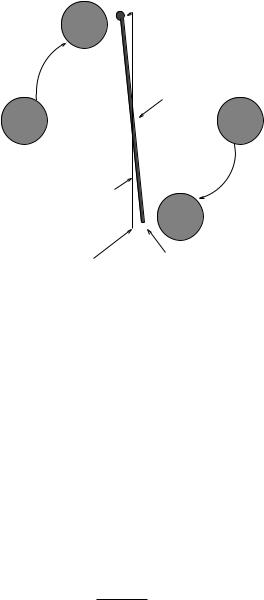
Henry Cavendish made the first direct measurement of G using a torsional pendulum – basically a barbell suspended by a very thin, strong thread – and some really massive balls whose relative position could be smoothly adjusted to bring them closer to and farter from the barbell balls. As you can imagine, it takes very little torque to twist a long thread from its equilibrium angle to a new one, so this apparatus has – when utilized by someone with a great deal of patience, using a light source and a mirror to further amplify the resolution of the twist angle – proven to be su ciently sensitive to measure the tiny forces required to determine G, even to some reasonable precision.
Using this apparatus, he was able to find G and hence to “weigh the earth” (find ME ). By measuring θ as a function of the distance r measured between the centers of the balls, and calibrating
Week 12: Gravity |
501 |
m
M
M
Δθ
equilibrium position (no mass M)
torsional pivot
M
M m
equilibrium position when attracted by mass M
Figure 147: The apparatus associated with the Cavendish experiment, which established the first accurate estimates for G and thereby “weighed the Earth”, the Sun, and many of the other objects we could see in the sky.
the torsional response of the string using known forces, he managed to get 6.754 (vs 6.673 currently accepted) ×10−11 N-m2/kg2. This is within just about one percent. Not bad!
12.4.1: Spheres, Shells, General Mass Distributions
So far, our empirically founded expression for gravitational force (and by inheritance, field) applies only to spherically symmetric mass distributions – planets and stars, which are generally almost perfectly round because of the gravitational field – or particles small enough that they can be treated like spheres. Our pathway towards the gravitational field of more general distributions of mass starts by formulating the field of a single point-like chunk of mass in such a distribution:
d~g = − |
G dm0 |
(~r − ~r0) |
(1052) |
|~r − ~r0|3 |
This equation can be integrated as usual over an arbitrary mass distribution using the usual connection: The mass of each chunk is the mass per unit volume times the volume of the chunk, or
dm = ρdV0. |
|
|
|
~g = −Z |
G ρ dV0 |
(~r − ~r0) |
(1053) |
|~r − ~r0|3 |
|||
where for example dV0 = dx0dy0dz0 (Cartesian) or dV0 = r02 sin(θ0)dθ0dφ0dr0 |
(Sphereical Polar) |
etc. This integral is not always easy, but it can generally be done very accurately, if necessary numerically. In simple cases we can actually do the calculus and evaluate the integral.
In this part of this course, we will avoid doing the integral, although we will tackle many examples of doing it in simple cases next semester. We will content ourselves with learning the following True Facts about the gravitational field:
• The gravitational field produced by a (thin) spherically symmetric shell of mass M vanishes inside the shell.