

- •Preface
- •Textbook Layout and Design
- •Preliminaries
- •See, Do, Teach
- •Other Conditions for Learning
- •Your Brain and Learning
- •The Method of Three Passes
- •Mathematics
- •Summary
- •Homework for Week 0
- •Summary
- •1.1: Introduction: A Bit of History and Philosophy
- •1.2: Dynamics
- •1.3: Coordinates
- •1.5: Forces
- •1.5.1: The Forces of Nature
- •1.5.2: Force Rules
- •Example 1.6.1: Spring and Mass in Static Force Equilibrium
- •1.7: Simple Motion in One Dimension
- •Example 1.7.1: A Mass Falling from Height H
- •Example 1.7.2: A Constant Force in One Dimension
- •1.7.1: Solving Problems with More Than One Object
- •Example 1.7.4: Braking for Bikes, or Just Breaking Bikes?
- •1.8: Motion in Two Dimensions
- •Example 1.8.1: Trajectory of a Cannonball
- •1.8.2: The Inclined Plane
- •Example 1.8.2: The Inclined Plane
- •1.9: Circular Motion
- •1.9.1: Tangential Velocity
- •1.9.2: Centripetal Acceleration
- •Example 1.9.1: Ball on a String
- •Example 1.9.2: Tether Ball/Conic Pendulum
- •1.9.3: Tangential Acceleration
- •Homework for Week 1
- •Summary
- •2.1: Friction
- •Example 2.1.1: Inclined Plane of Length L with Friction
- •Example 2.1.3: Find The Minimum No-Skid Braking Distance for a Car
- •Example 2.1.4: Car Rounding a Banked Curve with Friction
- •2.2: Drag Forces
- •2.2.1: Stokes, or Laminar Drag
- •2.2.2: Rayleigh, or Turbulent Drag
- •2.2.3: Terminal velocity
- •Example 2.2.1: Falling From a Plane and Surviving
- •2.2.4: Advanced: Solution to Equations of Motion for Turbulent Drag
- •Example 2.2.3: Dropping the Ram
- •2.3.1: Time
- •2.3.2: Space
- •2.4.1: Identifying Inertial Frames
- •Example 2.4.1: Weight in an Elevator
- •Example 2.4.2: Pendulum in a Boxcar
- •2.4.2: Advanced: General Relativity and Accelerating Frames
- •2.5: Just For Fun: Hurricanes
- •Homework for Week 2
- •Week 3: Work and Energy
- •Summary
- •3.1: Work and Kinetic Energy
- •3.1.1: Units of Work and Energy
- •3.1.2: Kinetic Energy
- •3.2: The Work-Kinetic Energy Theorem
- •3.2.1: Derivation I: Rectangle Approximation Summation
- •3.2.2: Derivation II: Calculus-y (Chain Rule) Derivation
- •Example 3.2.1: Pulling a Block
- •Example 3.2.2: Range of a Spring Gun
- •3.3: Conservative Forces: Potential Energy
- •3.3.1: Force from Potential Energy
- •3.3.2: Potential Energy Function for Near-Earth Gravity
- •3.3.3: Springs
- •3.4: Conservation of Mechanical Energy
- •3.4.1: Force, Potential Energy, and Total Mechanical Energy
- •Example 3.4.1: Falling Ball Reprise
- •Example 3.4.2: Block Sliding Down Frictionless Incline Reprise
- •Example 3.4.3: A Simple Pendulum
- •Example 3.4.4: Looping the Loop
- •3.5: Generalized Work-Mechanical Energy Theorem
- •Example 3.5.1: Block Sliding Down a Rough Incline
- •Example 3.5.2: A Spring and Rough Incline
- •3.5.1: Heat and Conservation of Energy
- •3.6: Power
- •Example 3.6.1: Rocket Power
- •3.7: Equilibrium
- •3.7.1: Energy Diagrams: Turning Points and Forbidden Regions
- •Homework for Week 3
- •Summary
- •4.1: Systems of Particles
- •Example 4.1.1: Center of Mass of a Few Discrete Particles
- •4.1.2: Coarse Graining: Continuous Mass Distributions
- •Example 4.1.2: Center of Mass of a Continuous Rod
- •Example 4.1.3: Center of mass of a circular wedge
- •4.2: Momentum
- •4.2.1: The Law of Conservation of Momentum
- •4.3: Impulse
- •Example 4.3.1: Average Force Driving a Golf Ball
- •Example 4.3.2: Force, Impulse and Momentum for Windshield and Bug
- •4.3.1: The Impulse Approximation
- •4.3.2: Impulse, Fluids, and Pressure
- •4.4: Center of Mass Reference Frame
- •4.5: Collisions
- •4.5.1: Momentum Conservation in the Impulse Approximation
- •4.5.2: Elastic Collisions
- •4.5.3: Fully Inelastic Collisions
- •4.5.4: Partially Inelastic Collisions
- •4.6: 1-D Elastic Collisions
- •4.6.1: The Relative Velocity Approach
- •4.6.2: 1D Elastic Collision in the Center of Mass Frame
- •4.7: Elastic Collisions in 2-3 Dimensions
- •4.8: Inelastic Collisions
- •Example 4.8.1: One-dimensional Fully Inelastic Collision (only)
- •Example 4.8.2: Ballistic Pendulum
- •Example 4.8.3: Partially Inelastic Collision
- •4.9: Kinetic Energy in the CM Frame
- •Homework for Week 4
- •Summary
- •5.1: Rotational Coordinates in One Dimension
- •5.2.1: The r-dependence of Torque
- •5.2.2: Summing the Moment of Inertia
- •5.3: The Moment of Inertia
- •Example 5.3.1: The Moment of Inertia of a Rod Pivoted at One End
- •5.3.1: Moment of Inertia of a General Rigid Body
- •Example 5.3.2: Moment of Inertia of a Ring
- •Example 5.3.3: Moment of Inertia of a Disk
- •5.3.2: Table of Useful Moments of Inertia
- •5.4: Torque as a Cross Product
- •Example 5.4.1: Rolling the Spool
- •5.5: Torque and the Center of Gravity
- •Example 5.5.1: The Angular Acceleration of a Hanging Rod
- •Example 5.6.1: A Disk Rolling Down an Incline
- •5.7: Rotational Work and Energy
- •5.7.1: Work Done on a Rigid Object
- •5.7.2: The Rolling Constraint and Work
- •Example 5.7.2: Unrolling Spool
- •Example 5.7.3: A Rolling Ball Loops-the-Loop
- •5.8: The Parallel Axis Theorem
- •Example 5.8.1: Moon Around Earth, Earth Around Sun
- •Example 5.8.2: Moment of Inertia of a Hoop Pivoted on One Side
- •5.9: Perpendicular Axis Theorem
- •Example 5.9.1: Moment of Inertia of Hoop for Planar Axis
- •Homework for Week 5
- •Summary
- •6.1: Vector Torque
- •6.2: Total Torque
- •6.2.1: The Law of Conservation of Angular Momentum
- •Example 6.3.1: Angular Momentum of a Point Mass Moving in a Circle
- •Example 6.3.2: Angular Momentum of a Rod Swinging in a Circle
- •Example 6.3.3: Angular Momentum of a Rotating Disk
- •Example 6.3.4: Angular Momentum of Rod Sweeping out Cone
- •6.4: Angular Momentum Conservation
- •Example 6.4.1: The Spinning Professor
- •6.4.1: Radial Forces and Angular Momentum Conservation
- •Example 6.4.2: Mass Orbits On a String
- •6.5: Collisions
- •Example 6.5.1: Fully Inelastic Collision of Ball of Putty with a Free Rod
- •Example 6.5.2: Fully Inelastic Collision of Ball of Putty with Pivoted Rod
- •6.5.1: More General Collisions
- •Example 6.6.1: Rotating Your Tires
- •6.7: Precession of a Top
- •Homework for Week 6
- •Week 7: Statics
- •Statics Summary
- •7.1: Conditions for Static Equilibrium
- •7.2: Static Equilibrium Problems
- •Example 7.2.1: Balancing a See-Saw
- •Example 7.2.2: Two Saw Horses
- •Example 7.2.3: Hanging a Tavern Sign
- •7.2.1: Equilibrium with a Vector Torque
- •Example 7.2.4: Building a Deck
- •7.3: Tipping
- •Example 7.3.1: Tipping Versus Slipping
- •Example 7.3.2: Tipping While Pushing
- •7.4: Force Couples
- •Example 7.4.1: Rolling the Cylinder Over a Step
- •Homework for Week 7
- •Week 8: Fluids
- •Fluids Summary
- •8.1: General Fluid Properties
- •8.1.1: Pressure
- •8.1.2: Density
- •8.1.3: Compressibility
- •8.1.5: Properties Summary
- •Static Fluids
- •8.1.8: Variation of Pressure in Incompressible Fluids
- •Example 8.1.1: Barometers
- •Example 8.1.2: Variation of Oceanic Pressure with Depth
- •8.1.9: Variation of Pressure in Compressible Fluids
- •Example 8.1.3: Variation of Atmospheric Pressure with Height
- •Example 8.2.1: A Hydraulic Lift
- •8.3: Fluid Displacement and Buoyancy
- •Example 8.3.1: Testing the Crown I
- •Example 8.3.2: Testing the Crown II
- •8.4: Fluid Flow
- •8.4.1: Conservation of Flow
- •Example 8.4.1: Emptying the Iced Tea
- •8.4.3: Fluid Viscosity and Resistance
- •8.4.4: A Brief Note on Turbulence
- •8.5: The Human Circulatory System
- •Example 8.5.1: Atherosclerotic Plaque Partially Occludes a Blood Vessel
- •Example 8.5.2: Aneurisms
- •Homework for Week 8
- •Week 9: Oscillations
- •Oscillation Summary
- •9.1: The Simple Harmonic Oscillator
- •9.1.1: The Archetypical Simple Harmonic Oscillator: A Mass on a Spring
- •9.1.2: The Simple Harmonic Oscillator Solution
- •9.1.3: Plotting the Solution: Relations Involving
- •9.1.4: The Energy of a Mass on a Spring
- •9.2: The Pendulum
- •9.2.1: The Physical Pendulum
- •9.3: Damped Oscillation
- •9.3.1: Properties of the Damped Oscillator
- •Example 9.3.1: Car Shock Absorbers
- •9.4: Damped, Driven Oscillation: Resonance
- •9.4.1: Harmonic Driving Forces
- •9.4.2: Solution to Damped, Driven, Simple Harmonic Oscillator
- •9.5: Elastic Properties of Materials
- •9.5.1: Simple Models for Molecular Bonds
- •9.5.2: The Force Constant
- •9.5.3: A Microscopic Picture of a Solid
- •9.5.4: Shear Forces and the Shear Modulus
- •9.5.5: Deformation and Fracture
- •9.6: Human Bone
- •Example 9.6.1: Scaling of Bones with Animal Size
- •Homework for Week 9
- •Week 10: The Wave Equation
- •Wave Summary
- •10.1: Waves
- •10.2: Waves on a String
- •10.3: Solutions to the Wave Equation
- •10.3.1: An Important Property of Waves: Superposition
- •10.3.2: Arbitrary Waveforms Propagating to the Left or Right
- •10.3.3: Harmonic Waveforms Propagating to the Left or Right
- •10.3.4: Stationary Waves
- •10.5: Energy
- •Homework for Week 10
- •Week 11: Sound
- •Sound Summary
- •11.1: Sound Waves in a Fluid
- •11.2: Sound Wave Solutions
- •11.3: Sound Wave Intensity
- •11.3.1: Sound Displacement and Intensity In Terms of Pressure
- •11.3.2: Sound Pressure and Decibels
- •11.4: Doppler Shift
- •11.4.1: Moving Source
- •11.4.2: Moving Receiver
- •11.4.3: Moving Source and Moving Receiver
- •11.5: Standing Waves in Pipes
- •11.5.1: Pipe Closed at Both Ends
- •11.5.2: Pipe Closed at One End
- •11.5.3: Pipe Open at Both Ends
- •11.6: Beats
- •11.7: Interference and Sound Waves
- •Homework for Week 11
- •Week 12: Gravity
- •Gravity Summary
- •12.1: Cosmological Models
- •12.2.1: Ellipses and Conic Sections
- •12.4: The Gravitational Field
- •12.4.1: Spheres, Shells, General Mass Distributions
- •12.5: Gravitational Potential Energy
- •12.6: Energy Diagrams and Orbits
- •12.7: Escape Velocity, Escape Energy
- •Example 12.7.1: How to Cause an Extinction Event
- •Homework for Week 12
502 |
|
|
Week 12: Gravity |
• The gravitational field produced by this same shell equals the usual |
|
||
~g(~r) = − |
G M |
rˆ |
(1054) |
|
|||
r2 |
|||
outside of the shell. As a consequence the field outside of any spherically symmetric distribution of mass is just
~g(~r) = − |
G M |
rˆ |
(1055) |
r2 |
These two results can be proven by direct integration or by using Gauss’s Law for the gravitational field (using methodology developed next semester for the electrostatic field). The latter is so easy that it is hardly worth the time to learn the former for this special case.
Note well the most important consequence for our purposes in the homework of this rule is that when we descend a tunnel into a uniformly dense planet, the gravity will diminish as we are only pulled down by the mass inside our radius. This means that the gravitational field we experience is:
~g(~r) = − |
G M (r) |
rˆ |
(1056) |
r2 |
where M (r) = ρ4πr3/3 for a uniform density, something more complicated in cases where the density itself changes with r. You will use this expression in several homework problems.
12.5: Gravitational Potential Energy
W t = 0
W
12 |
|
|
|
B |
|
A |
W |
|
r W t = 0 |
||
12 |
||
1 |
r2 |
|
|
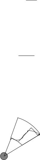
Figure 148: A crude illustration of how one can show the gravitational force to be conservative (so that the work done by the force is independent of the path taken between two points), permitting the evaluation of a potential energy function.
If you examine figure 148 above, and note that the force is always “down” along ~r, it is easy to conclude that gravity must be a conservative force. Gravity produced by some (spherically symmetric or point-like) mass does work on another mass only when that mass is moved in or out along ~r connecting them; moving at right angles to this along a surface of constant radius r involves no gravitational work. Any path between two points near the source can be broken up into approximating segments parallel to ~r and perpendicular to ~r at each point, and one can make the approximation as good as you like by choosing small enough segments.
This permits us to easily compute the gravitational potential energy as the negative work done

Week 12: Gravity
moving a mass m from a reference position ~r0 to a final position ~r:
U (r) = −Zr0 F~ |
· d~r |
|
|
|
|||||||
|
|
|
r |
|
|
|
|
|
|
|
|
= |
−Zr0 |
− |
|
|
r2 |
dr |
|
||||
|
|
|
r |
|
GM m |
|
|||||
= |
−( |
GM m |
GM m |
|
|||||||
|
|
|
|
− |
|
|
) |
||||
|
r |
|
|
r0 |
|||||||
|
GM m GM m |
|
|||||||||
= |
− |
|
|
|
+ |
|
|
|
|
||
|
r |
|
|
r0 |
|
||||||
503
(1057)
(1058)
(1059)
(1060)
Note that the potential energy function depends only on the scalar magnitude of ~r0 and ~r, and that r0 is in the end the radius of an arbitrary point where we define the potential energy to be zero.
By convention, unless there is a good reason to gravitational potential energy function to be at r0 =
choose otherwise, we require the zero of the ∞. Thus:
U (r) = − |
GM m |
(1061) |
r |
Note that since energy in some sense is more fundamental than force (the latter is the negative derivative of the former) we could just as easily have learned Newton’s Law of Gravitation directly as this scalar potential energy function and then evaluated the force by taking its negative gradient (multidimensional derivative).
The most important thing to note about this function is that it is always negative. Recall that the force points in the direction that the potential energy decreases most strongly in. Since U (r) is negative and gets larger in magnitude for smaller r, gravitation (correctly) points down to smaller r where the potential energy is “smaller” (more negative).
The potential energy function will be very useful to us when we wish to consider things like escape velocity/energy, killer asteroids, energy diagrams, and orbits. Let’s start with energy diagrams and orbits.
12.6: Energy Diagrams and Orbits
Let’s write the total energy of a particle moving in a gravitational field in a clever way that isolates the radial kinetic energy:
Etot = |
1 |
mv2 |
− |
GM m |
|
|
|
|
(1062) |
||||
|
|
|
|
|
|
|
|
|
|
||||
|
2 |
|
r |
|
|
|
|
||||||
= |
1 |
mvr2 |
+ |
1 |
mvt2 − |
GM m |
|
(1063) |
|||||
|
|
|
|
|
|
|
|||||||
|
2 |
2 |
r |
|
|||||||||
= |
1 |
mvr2 |
+ |
1 |
(mvtr)2 − |
GM m |
(1064) |
||||||
|
|
|
|
||||||||||
|
2 |
2mr2 |
r |
||||||||||
|
1 |
mvr2 |
|
|
L2 |
GM m |
|
|
|||||
= |
|
|
+ |
|
− |
|
|
|
(1065) |
||||
|
2 |
2mr2 |
r |
|
|||||||||
= |
|
1 |
mvr2 |
+ Ue (r) |
|
|
|
|
(1066) |
||||
2 |
|
|
|
|
|||||||||
|
|
|
|
|
|
|
|
|
|
|
|
||
In this equation, 12 mvr2 is the radial kinetic energy, and
|
L2 |
GM m |
|
|
Ue (r) = |
|
− |
|
(1067) |
2mr2 |
r |
|||
is the radial potential energy plus the rotational kinetic energy of the orbiting particle, formed out of the transverse velocity vt as Krot = 12 mvt2 = L2/2mr2. If we plot the e ective potential (and its pieces) we get a one-dimensional radial energy plot as illustrated in figure 149.