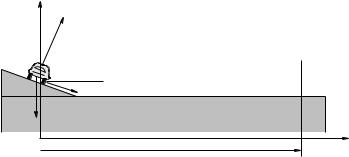
which (if you think about it) makes both dimensional and physical sense. In terms of the given numbers, m2 > musm1 = 4 kg is enough so that the weight of the second mass will make the whole system move. Note that the tension T = m2g = 40 Newtons, from Fx2 (now that we know m2).

Similarly, in the second pair of questions m2 is larger than this minimum, so m1 will slide to the right as m2 falls. We will have to solve Newton’s Second Law for both masses in order to obtain the non-zero acceleration to the right and down, respectively:

If we substitute the fixed value for fk = µkN = µkm1g and then add the two x equations once again (using the fact that both masses have the same acceleration because the string is unstretchable as noted in our original construction of round-the-corner coordinates), the tension T cancels and we get:

is the constant acceleration.

This makes sense! The string forms an “internal force” not unlike the molecular forces that glue the many tiny components of each block together. As long as the two move together, these internal forces do not contribute to the collective motion of the system any more than you can pick yourself up by your own shoestrings! The net force “along x” is just the weight of m2 pulling one way, and the force of kinetic friction pulling the other. The sum of these two forces equals the total mass times the acceleration!

Solving for v(t) and x(t) (for either block) should now be easy and familiar. So should finding the time it takes for the blocks to move one meter, and substituting this time into v(t) to find out how fast they are moving at this time. Finally, one can substitute a into either of the two equations of motion involving T and solve for T . In general you should find that T is less than the weight of the second mass, so that the net force on this mass is not zero and accelerates it downward. The tension T can never be negative (as drawn) because strings can never push an object, only pull.

Basically, we are done. We know (or can easily compute) anything that can be known about this system.

Example 2.1.3: Find The Minimum No-Skid Braking Distance for a Car

One of the most important everyday applications of our knowledge of static versus kinetic friction is in anti-lock brake systems (ABS)53 ABS brakes are implemented in every car sold in the European Union (since 2007) and are standard equipment in almost every car sold in the United States, where for reasons known only to congress it has yet to be formally mandated. This is in spite of the fact that road tests show that on average, stopping distances for ABS-equipped cars are some 18 to 35% shorter than non-ABS equipped cars, for all but the most skilled drivers (who still find it di cult to actually beat ABS stopping distances but who can equal them).

One small part of the reason may be that ABS braking “feels strange” as the car pumps the brakes for you 10-16 times per second, making it “pulse” as it stops. This causes drivers unprepared

53Wikipedia: http://www.wikipedia.org/wiki/Anti-lock Braking System.

Figure 19: Stopping a car with and without locking the brakes and skidding. The coordinate system (not drawn) is x parallel to the ground, y perpendicular to the ground, and the origin in both cases is at the point where the car begins braking. In panel a), the anti-lock brakes do not lock and the car is stopped with the maximum force of static friction. In panel b) the brakes lock and the car skids to a stop, slowed by kinetic/sliding friction.

for the feeling to back o of the brake pedal and not take full advantage of the ABS feature, but of course the simpler and better solution is for drivers to educate themselves on the feel of anti-lock brakes in action under safe and controlled conditions and then trust them.

This problem is designed to help you understand why ABS-equipped cars are “better” (safer) than non-ABS-equipped cars, and why you should rely on them to help you stop a car in the minimum possible distance. We achieve this by answer the following questions:

Find the minimum braking distance of a car travelling at speed v0 30 m/sec running on tires with µs = 0.5 and µk = 0.3:

a)equipped with ABS such that the tires do not skid, but rather roll (so that they exert the maximum static friction only);

b)the same car, but without ABS and with the wheels locked in a skid (kinetic friction only)

c)Evaluate these distances for v0 = 30 meters/second ( 67 mph), and both for µs = 0.8, µk = 0.7 (reasonable values, actually, for good tires on dry pavement) and for µs = 0.7, µk = 0.3 (not unreasonable values for wet pavement). The latter are, however, highly variable, depending on the kind and conditions of the treads on your car (which provide channels for water to be displaced as a thin film of water beneath the treads lubricates the point of contact between the tire and the road. With luck they will teach you why you should slow down and allow the distance between your vehicle and the next one to stretch out when driving in wet, snowy, or icy conditions.

To answer all of these questions, it su ces to evalute the acceleration of the car given either fsmax = µsN = µsmg (for a car being stopped by peak static friction via ABS) and fk = µkN =

a)The normal force exerted by the road on the car.

b)The force of static friction exerted by the road on the tires.

c)The range of speeds for which the car can round the curve successfully (without sliding up or down the incline).

Note that we don’t know fs, but we are certain that it must be less than or equal to µsN in order for the car to successfully round the curve (the third question). To be able to formulate the range problem, though, we have to find the normal force (in terms of the other/given quantities and the force exerted by static friction (in terms of the other quantities), so we start with that.

As always, the only thing we really know is our dynamical principle – Newton’s Second Law – plus our knowledge of the force rules involved plus our experience and intuition, which turn out to be crucial in setting up this problem.

For example, what direction should fs point? Imagine that the inclined roadway is coated with frictionless ice and the car is sitting on it (almost) at rest (for a finite but tiny v → 0). What will happen (if µs = µk = 0)? Well, obviously it will slide down the hill which doesn’t qualify as ‘rounding the curve’ at a constant height on the incline. Now imagine that the car is travelling at an enormous v; what will happen? The car will skid o of the road to the outside, of course. We know (and fear!) that from our own experience rounding curves too fast.

We now have two di erent limiting behaviors – in the first case, to round the curve friction has to keep the car from sliding down at low speeds and hence must point up the incline; in the second case, to round the curve friction has to point down to keep the car from skidding up and o of the road.

We have little choice but to pick one of these two possibilities, solve the problem for that possibility, and then solve it again for the other (which should be as simple as changing the sign of fs in the algebra. I therefore arbitrarily picked fs pointing down (and parallel to, remember) the incline, which will eventually give us the upper limit on the speed v with which we can round the curve.

~

As always we use coordinates lined up with the eventual direction of F tot and the actual acceleration of the car: +x parallel to the ground (and the plane of the circle of movement with radius R).

y

(where so far fs is not its maximum value, it is merely whatever it needs to be to make the car round the curve for a v presumed to be in range) and solve the y equation for N :