

110 Week 2: Newton’s Laws: Continued
The number Cd is called the drag coe cient and is a dimensionless number that depends on relative speed, flow direction, object position, object size, fluid viscosity and fluid density. In other words, the expression above is only valid in certain domains of all of these properties where Cd is slowly varying and can be thought of as a “constant”! Hence we can say that for a sphere moving
through still air at speeds where turbulent drag is dominant it is around 0.47 ≈ 0.5, or: |
|
||
bt ≈ |
1 |
ρπR2 |
(175) |
4 |
|||
which one can compare to bl = 6µπR for the Stokes drag of the same sphere, moving much slower.
To get a feel for non-spherical objects, blu convex objects like potatoes or cars or people have drag coe cients close to but a bit more or less than 0.5, while highly blu objects might have a drag coe cient over 1.0 and truly streamlined objects might have a drag coe cient as low as 0.04.
As one can see, the functional complexity of the actual non-constant drag coe cient Cd even for such a simple object as a sphere has to manage the entire transition from laminar drag force for low velocities/Reynold’s numbers to turbulent drag for high velocites/Reynold’s numbers, so that at speeds in between the drag force is at best a function of a non-integer power of v in between 1 and 2 or some arcane mixture of form drag and skin friction. We will pretty much ignore this transition. It is just too damned di cult for us to mess with, although you should certainly be aware that it is there.
You can see that in our actual expression for the drag force above, as promised, we have simplified things even more and express all of this dependence – ρ, µ, size and shape and more – wrapped up in the turbulent dimensioned constant bt, which one can think of as an overall turbulent drag coe cient that plays the same general role as the laminar drag coe cient bl we similarly defined above. However, it is impossible for the heuristic descriptors bl and bt to be the same for Stokes’ and turbulent drag – they don’t even have the same units – and for most objects most of the time the total drag is some sort of mixture of these limiting forces, with one or the other (probably) dominant.
As you can see, drag forces are complicated! In the end, they turn out to be most useful (to us) as heuristic rules with drag coe cients bl or bt given so that we can see what we can reasonably compute or estimate in these limits.
2.2.3: Terminal velocity
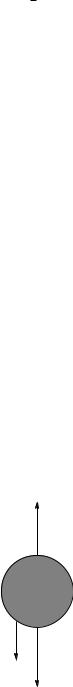
Fd
v
mg
Figure 22: A simple object falling through a fluid experiences a drag force that increasingly cancels the force of gravity as the object accelerates until a terminal velocity vt is asymptotically reached. For blu objects such as spheres, the Fd = −bv2 force rule is usually appropriate.
One immediate consequence of this is that objects dropped in a gravitational field in fluids such as air or water do not just keep speeding up ad infinitum. When they are dropped from rest, at first

Week 2: Newton’s Laws: Continued |
111 |
their speed is very low and drag forces may well be negligible58. The gravitational force accelerates them downward and their speed gradually increases.
As it increases, however, the drag force in all cases increases as well. For many objects the drag forces will quickly transition over to turbulent drag, with a drag force magnitude of btv2. For others, the drag force may remain Stokes’ drag, with a drag force magnitude of blv (in both cases opposing the directioin of motion through the fluid). Eventually, the drag force will balance the gravitational force and the object will no longer accelerate. It will fall instead at a constant speed. This speed is called the terminal velocity.
It is extremely easy to compute the terminal velocity for a falling object, given the form of its drag force rule. It is the velocity where the net force on the object vanishes. If we choose a coordinate system with “down” being e.g. x positive (so gravity and the velocity are both positive pointing down) we can write either:
mg − blvt |
= max = 0 |
or |
||||||
vt |
= |
mg |
(176) |
|||||
|
bl |
|
||||||
|
|
|
|
|||||
(for Stokes’ drag) or |
|
|
|
|
|
|
|
|
mg − btvt2 |
= |
max = 0 |
and |
|||||
vt |
= |
r |
bt |
|
(177) |
|||
|
|
|
|
mg |
|
|
||
|
|
|
|
|
|
|
|
|
for turbulent drag.
We expect vx(t) to asymptotically approach vt with time. Rather than draw a generic asymptotic curve (which is easy enough, just start with the slope of v being g and bend the curve over to smoothly approach vt), we will go ahead and see how to solve the equations of motion for at least the two limiting (and common) cases of Stokes’ and turbulent drag.
The entire complicated set of drag formulas above can be reduced to the following “rule of thumb” that applies to objects of water-like density that have sizes such that turbulent drag determines their terminal velocity – raindrops, hail, live animals (including humans) falling in air just above sea level near the surface of the Earth. In this case terminal velocity is roughly equal to
√ |
|
vt = 90 d |
(178) |
where d is the characteristic size of the object in meters.
For a human body d ≈ 0.6 so vt ≈ 70 meters per second or 156 miles per hour. However, if one falls in a blu position, one can reduce this to anywhere from 40 to 55 meters per second, say 90 to 120 miles per hour.
Note that the characteristic size of a small animal such as a squirrel or a cat might be 0.05 (squirrel) to 0.1 (cat). Terminal velocity for a cat is around 28 meters per second, lower if the cat falls in a blu position (say, 50 to 60 mph) and for a squirrel in a blu position it might be as low as 10 to 20 mph. Smaller animals – especially ones with large bushy tails or skin webs like those observed in the flying squirrel 59 – have a much lower terminal velocity than (say) humans and hence have a much better chance of survival. One rather imagines that this provided a direct evolutionary path to actual flight for small animals that lived relatively high above the ground in arboreal niches.
58In air and other low viscosity, low density compressible gases they probably are; in water or other viscous, dense, incompressible liquids they may not be.
59Wikipedia: http://www.wikipedia.org/wiki/Flying Squirrel. A flying squirrel doesn’t really fly – rather it skydives
in a highly blu position so that it can glide long transverse distances and land with a very low terminal velocity.

112 |
Week 2: Newton’s Laws: Continued |
Example 2.2.1: Falling From a Plane and Surviving
As noted above, the terminal velocity for humans in free fall near the Earth’s surface is (give or take, depending on whether you are falling in a streamlined swan dive or falling in a blu skydiver’s belly flop position) anywhere from 40 to 70 meters per second (90-155 miles per hour). Amazingly, humans can survive60 collisions at this speed.
The trick is to fall into something soft and springy that gradually slows you from high speed to zero without ever causing the deceleration force to exceed 100 times your weight, applied as uniformly as possible to parts of your body you can live without such as your legs (where your odds go up the smalller this multiplier is, of course). It is pretty simple to figure out what kinds of things might do.
Suppose you fall from a large height (long enough to reach terminal velocity) to hit a haystack of height H that exerts a nice, uniform force to slow you down all the way to the ground, smoothly compressing under you as you fall. In that case, your initial velocity at the top is vt, down. In order to stop you before y = 0 (the ground) you have to have a net acceleration −a such that:
v(tg ) |
= |
0 |
= vt − atg |
1 |
|
(179) |
|
y(tg ) |
= |
0 |
= H − vttg − |
atg2 |
(180) |
||
|
|||||||
2 |
If we solve the first equation for tg (something we have done many times now) and substitute it into the second and solve for the magnitude of a, we will get:
− vt2 |
= −2aH or |
|
|
|
|
|||
|
|
|
v2 |
|
|
|
|
|
a |
= |
|
t |
|
|
|
|
(181) |
2H |
|
|
|
|||||
|
|
|
|
|
|
|||
We know also that |
|
|
|
|
|
|
|
|
Fhaystack − mg = ma |
|
|
|
(182) |
||||
or |
|
|
|
|
µ |
2H + g¶ |
(183) |
|
Fhaystack = ma + mg = m(a + g) = mg′ = m |
||||||||
|
|
|
|
|
|
v2 |
|
|
|
|
|
|
|
|
t |
|
|
Let’s suppose the haystack was H = 1.25 meter high and, because you cleverly landed on it in a “blu ” position to keep vt as small as possible, you start at the top moving at only vt = 50 meters per second. Then g′ = a + g is approximately 1009.8 meters/second2, 103 ‘gees’, and the force the haystack must exert on you is 103 times your normal weight. You actually have a small chance of surviving this stopping force, but it isn’t a very large one.
To have a better chance of surviving, one needs to keep the g-force under 100, ideally well under 100, although a very few people are known to have survived 100 g accelerations in e.g. race car crashes. Since the “haystack” portion of the acceleration needed is inversely proportional to H we can see that a 2.5 meter haystack would lead to 51 gees, a 5 meter haystack would lead to 26 gees, and a 10 meter haystack would lead to a mere 13.5 gees, nothing worse than some serious bruising. If you want to get up and walk to your press conference, you need a haystack or palette at the mattress factory or thick pine forest that will uniformly slow you over something like 10 or more meters. I myself would prefer a stack of pillows at least 40 meters high... but then I have been known to crack a rib just falling a meter or so playing basketball.
The amazing thing is that a number of people have been reliably documented61 to have survived just such a fall, often with a stopping distance of only a very few meters if that, from falls as high
60Wikipedia: http://www.wikipedia.org/wiki/Free fall#Surviving falls. ...and have survived...
61http://www.greenharbor.com/ folder/ research.html This website contains ongoing and constantly updated links
to contemporary survivor stories as well as historical ones. It’s a fun read.

Week 2: Newton’s Laws: Continued |
113 |
as 18,000 feet. Sure, they usually survive with horrible injuries, but in a very few cases, e.g. falling into a deep bank of snow at a grazing angle on a hillside, or landing while strapped into an airline seat that crashed down through a thick forest canopy they haven’t been particularly badly hurt...
Kids, don’t try this at home! But if you ever do happen to fall out of an airplane at a few thousand feet, isn’t it nice that your physics class helps you have the best possible chance at surviving?
Example 2.2.2: Solution to Equations of Motion for Stokes’ Drag
We don’t have to work very hard to actually find and solve the equations of motion for a streamlined object that falls subject to a Stokes’ drag force.
We begin by writing the total force equation for an object falling down subject to near-Earth gravity and Stokes’ drag, with down being positive:
dv |
|
mg − bv = m dt |
(184) |
(where we’ve selected the down direction to be positive in this one-dimensional problem).
We rearrange this to put the velocity derivative by itself, factor out the coe cient of v on the right, divide through the v-term from the right, multiply through by dt, integrate both sides, exponentiate both sides, and set the constant of integration. Of course...
Was that too fast for you62? Like this:
|
|
|
|
|
|
dv |
|
|
|
|
|
|
|
|
b |
|
|
|
||||||
|
|
|
|
|
|
|
|
|
= |
g − |
|
v |
|
|
|
|||||||||
|
|
|
|
|
|
dt |
m |
´ |
|
|
||||||||||||||
|
|
|
|
|
|
dt |
= |
−m |
|
|
³v − b |
|
|
|||||||||||
|
|
|
|
|
|
dv |
|
|
|
b |
|
|
|
mg |
|
|
|
|||||||
|
|
dv |
|
|
= |
− |
b |
|
dt |
|
|
|
||||||||||||
|
|
|
|
|
|
|
|
|
|
|
|
|
|
|||||||||||
³ |
|
v − mgb |
m |
|
|
|
||||||||||||||||||
|
|
mg |
|
´ |
= |
− |
b |
|
|
|
|
|
|
|
|
|
||||||||
ln v − |
|
b |
|
|
m |
|
t + C |
|
|
|
||||||||||||||
|
|
|
|
|
mg |
|
|
|
|
b |
|
|
|
|
|
|
|
b |
||||||
|
v − |
|
|
|
|
|
|
= e− |
m |
teC = v0e− |
m |
t |
||||||||||||
|
|
|
b |
|
|
|||||||||||||||||||
|
|
|
|
v(t) = |
|
mg |
|
|
+ v0e− |
b |
t |
|
|
|
||||||||||
|
|
|
|
|
m |
|
|
|
||||||||||||||||
|
|
|
|
|
b |
|
|
|
|
|||||||||||||||
|
|
|
|
v(t) = |
|
b |
³1 − e−m t´ |
|||||||||||||||||
|
|
|
|
|
|
|
|
|
|
|
|
mg |
|
|
|
|
b |
|
|
|
||||
or
³ ´ v(t) = vt 1 − e−mb t
(185)
(186)
(where we used the fact that v(0) = 0 to set the constant of integration v0, which just happened to be vt, the terminal velocity!
Objects falling through a medium under the action of Stokes’ drag experience an exponential approach to a constant (terminal) velocity. This is an enormously useful piece of calculus to master; we will have a number of further opportunities to solve equations of motion this and next semester that are first order, linear, inhomogeneous ordinary di erential equations such as this one.
Given v(t) it isn’t too di cult to integrate again and find x(t), if we care to, but in this class we will usually stop here as x(t) has pieces that are both linear and exponential in t and isn’t as “pretty” as v(t) is.
62Just kidding! I know you (probably) have no idea how to do this. That’s why you’re taking this course!