- •Preface
- •Textbook Layout and Design
- •Preliminaries
- •See, Do, Teach
- •Other Conditions for Learning
- •Your Brain and Learning
- •The Method of Three Passes
- •Mathematics
- •Summary
- •Homework for Week 0
- •Summary
- •1.1: Introduction: A Bit of History and Philosophy
- •1.2: Dynamics
- •1.3: Coordinates
- •1.5: Forces
- •1.5.1: The Forces of Nature
- •1.5.2: Force Rules
- •Example 1.6.1: Spring and Mass in Static Force Equilibrium
- •1.7: Simple Motion in One Dimension
- •Example 1.7.1: A Mass Falling from Height H
- •Example 1.7.2: A Constant Force in One Dimension
- •1.7.1: Solving Problems with More Than One Object
- •Example 1.7.4: Braking for Bikes, or Just Breaking Bikes?
- •1.8: Motion in Two Dimensions
- •Example 1.8.1: Trajectory of a Cannonball
- •1.8.2: The Inclined Plane
- •Example 1.8.2: The Inclined Plane
- •1.9: Circular Motion
- •1.9.1: Tangential Velocity
- •1.9.2: Centripetal Acceleration
- •Example 1.9.1: Ball on a String
- •Example 1.9.2: Tether Ball/Conic Pendulum
- •1.9.3: Tangential Acceleration
- •Homework for Week 1
- •Summary
- •2.1: Friction
- •Example 2.1.1: Inclined Plane of Length L with Friction
- •Example 2.1.3: Find The Minimum No-Skid Braking Distance for a Car
- •Example 2.1.4: Car Rounding a Banked Curve with Friction
- •2.2: Drag Forces
- •2.2.1: Stokes, or Laminar Drag
- •2.2.2: Rayleigh, or Turbulent Drag
- •2.2.3: Terminal velocity
- •Example 2.2.1: Falling From a Plane and Surviving
- •2.2.4: Advanced: Solution to Equations of Motion for Turbulent Drag
- •Example 2.2.3: Dropping the Ram
- •2.3.1: Time
- •2.3.2: Space
- •2.4.1: Identifying Inertial Frames
- •Example 2.4.1: Weight in an Elevator
- •Example 2.4.2: Pendulum in a Boxcar
- •2.4.2: Advanced: General Relativity and Accelerating Frames
- •2.5: Just For Fun: Hurricanes
- •Homework for Week 2
- •Week 3: Work and Energy
- •Summary
- •3.1: Work and Kinetic Energy
- •3.1.1: Units of Work and Energy
- •3.1.2: Kinetic Energy
- •3.2: The Work-Kinetic Energy Theorem
- •3.2.1: Derivation I: Rectangle Approximation Summation
- •3.2.2: Derivation II: Calculus-y (Chain Rule) Derivation
- •Example 3.2.1: Pulling a Block
- •Example 3.2.2: Range of a Spring Gun
- •3.3: Conservative Forces: Potential Energy
- •3.3.1: Force from Potential Energy
- •3.3.2: Potential Energy Function for Near-Earth Gravity
- •3.3.3: Springs
- •3.4: Conservation of Mechanical Energy
- •3.4.1: Force, Potential Energy, and Total Mechanical Energy
- •Example 3.4.1: Falling Ball Reprise
- •Example 3.4.2: Block Sliding Down Frictionless Incline Reprise
- •Example 3.4.3: A Simple Pendulum
- •Example 3.4.4: Looping the Loop
- •3.5: Generalized Work-Mechanical Energy Theorem
- •Example 3.5.1: Block Sliding Down a Rough Incline
- •Example 3.5.2: A Spring and Rough Incline
- •3.5.1: Heat and Conservation of Energy
- •3.6: Power
- •Example 3.6.1: Rocket Power
- •3.7: Equilibrium
- •3.7.1: Energy Diagrams: Turning Points and Forbidden Regions
- •Homework for Week 3
- •Summary
- •4.1: Systems of Particles
- •Example 4.1.1: Center of Mass of a Few Discrete Particles
- •4.1.2: Coarse Graining: Continuous Mass Distributions
- •Example 4.1.2: Center of Mass of a Continuous Rod
- •Example 4.1.3: Center of mass of a circular wedge
- •4.2: Momentum
- •4.2.1: The Law of Conservation of Momentum
- •4.3: Impulse
- •Example 4.3.1: Average Force Driving a Golf Ball
- •Example 4.3.2: Force, Impulse and Momentum for Windshield and Bug
- •4.3.1: The Impulse Approximation
- •4.3.2: Impulse, Fluids, and Pressure
- •4.4: Center of Mass Reference Frame
- •4.5: Collisions
- •4.5.1: Momentum Conservation in the Impulse Approximation
- •4.5.2: Elastic Collisions
- •4.5.3: Fully Inelastic Collisions
- •4.5.4: Partially Inelastic Collisions
- •4.6: 1-D Elastic Collisions
- •4.6.1: The Relative Velocity Approach
- •4.6.2: 1D Elastic Collision in the Center of Mass Frame
- •4.7: Elastic Collisions in 2-3 Dimensions
- •4.8: Inelastic Collisions
- •Example 4.8.1: One-dimensional Fully Inelastic Collision (only)
- •Example 4.8.2: Ballistic Pendulum
- •Example 4.8.3: Partially Inelastic Collision
- •4.9: Kinetic Energy in the CM Frame
- •Homework for Week 4
- •Summary
- •5.1: Rotational Coordinates in One Dimension
- •5.2.1: The r-dependence of Torque
- •5.2.2: Summing the Moment of Inertia
- •5.3: The Moment of Inertia
- •Example 5.3.1: The Moment of Inertia of a Rod Pivoted at One End
- •5.3.1: Moment of Inertia of a General Rigid Body
- •Example 5.3.2: Moment of Inertia of a Ring
- •Example 5.3.3: Moment of Inertia of a Disk
- •5.3.2: Table of Useful Moments of Inertia
- •5.4: Torque as a Cross Product
- •Example 5.4.1: Rolling the Spool
- •5.5: Torque and the Center of Gravity
- •Example 5.5.1: The Angular Acceleration of a Hanging Rod
- •Example 5.6.1: A Disk Rolling Down an Incline
- •5.7: Rotational Work and Energy
- •5.7.1: Work Done on a Rigid Object
- •5.7.2: The Rolling Constraint and Work
- •Example 5.7.2: Unrolling Spool
- •Example 5.7.3: A Rolling Ball Loops-the-Loop
- •5.8: The Parallel Axis Theorem
- •Example 5.8.1: Moon Around Earth, Earth Around Sun
- •Example 5.8.2: Moment of Inertia of a Hoop Pivoted on One Side
- •5.9: Perpendicular Axis Theorem
- •Example 5.9.1: Moment of Inertia of Hoop for Planar Axis
- •Homework for Week 5
- •Summary
- •6.1: Vector Torque
- •6.2: Total Torque
- •6.2.1: The Law of Conservation of Angular Momentum
- •Example 6.3.1: Angular Momentum of a Point Mass Moving in a Circle
- •Example 6.3.2: Angular Momentum of a Rod Swinging in a Circle
- •Example 6.3.3: Angular Momentum of a Rotating Disk
- •Example 6.3.4: Angular Momentum of Rod Sweeping out Cone
- •6.4: Angular Momentum Conservation
- •Example 6.4.1: The Spinning Professor
- •6.4.1: Radial Forces and Angular Momentum Conservation
- •Example 6.4.2: Mass Orbits On a String
- •6.5: Collisions
- •Example 6.5.1: Fully Inelastic Collision of Ball of Putty with a Free Rod
- •Example 6.5.2: Fully Inelastic Collision of Ball of Putty with Pivoted Rod
- •6.5.1: More General Collisions
- •Example 6.6.1: Rotating Your Tires
- •6.7: Precession of a Top
- •Homework for Week 6
- •Week 7: Statics
- •Statics Summary
- •7.1: Conditions for Static Equilibrium
- •7.2: Static Equilibrium Problems
- •Example 7.2.1: Balancing a See-Saw
- •Example 7.2.2: Two Saw Horses
- •Example 7.2.3: Hanging a Tavern Sign
- •7.2.1: Equilibrium with a Vector Torque
- •Example 7.2.4: Building a Deck
- •7.3: Tipping
- •Example 7.3.1: Tipping Versus Slipping
- •Example 7.3.2: Tipping While Pushing
- •7.4: Force Couples
- •Example 7.4.1: Rolling the Cylinder Over a Step
- •Homework for Week 7
- •Week 8: Fluids
- •Fluids Summary
- •8.1: General Fluid Properties
- •8.1.1: Pressure
- •8.1.2: Density
- •8.1.3: Compressibility
- •8.1.5: Properties Summary
- •Static Fluids
- •8.1.8: Variation of Pressure in Incompressible Fluids
- •Example 8.1.1: Barometers
- •Example 8.1.2: Variation of Oceanic Pressure with Depth
- •8.1.9: Variation of Pressure in Compressible Fluids
- •Example 8.1.3: Variation of Atmospheric Pressure with Height
- •Example 8.2.1: A Hydraulic Lift
- •8.3: Fluid Displacement and Buoyancy
- •Example 8.3.1: Testing the Crown I
- •Example 8.3.2: Testing the Crown II
- •8.4: Fluid Flow
- •8.4.1: Conservation of Flow
- •Example 8.4.1: Emptying the Iced Tea
- •8.4.3: Fluid Viscosity and Resistance
- •8.4.4: A Brief Note on Turbulence
- •8.5: The Human Circulatory System
- •Example 8.5.1: Atherosclerotic Plaque Partially Occludes a Blood Vessel
- •Example 8.5.2: Aneurisms
- •Homework for Week 8
- •Week 9: Oscillations
- •Oscillation Summary
- •9.1: The Simple Harmonic Oscillator
- •9.1.1: The Archetypical Simple Harmonic Oscillator: A Mass on a Spring
- •9.1.2: The Simple Harmonic Oscillator Solution
- •9.1.3: Plotting the Solution: Relations Involving
- •9.1.4: The Energy of a Mass on a Spring
- •9.2: The Pendulum
- •9.2.1: The Physical Pendulum
- •9.3: Damped Oscillation
- •9.3.1: Properties of the Damped Oscillator
- •Example 9.3.1: Car Shock Absorbers
- •9.4: Damped, Driven Oscillation: Resonance
- •9.4.1: Harmonic Driving Forces
- •9.4.2: Solution to Damped, Driven, Simple Harmonic Oscillator
- •9.5: Elastic Properties of Materials
- •9.5.1: Simple Models for Molecular Bonds
- •9.5.2: The Force Constant
- •9.5.3: A Microscopic Picture of a Solid
- •9.5.4: Shear Forces and the Shear Modulus
- •9.5.5: Deformation and Fracture
- •9.6: Human Bone
- •Example 9.6.1: Scaling of Bones with Animal Size
- •Homework for Week 9
- •Week 10: The Wave Equation
- •Wave Summary
- •10.1: Waves
- •10.2: Waves on a String
- •10.3: Solutions to the Wave Equation
- •10.3.1: An Important Property of Waves: Superposition
- •10.3.2: Arbitrary Waveforms Propagating to the Left or Right
- •10.3.3: Harmonic Waveforms Propagating to the Left or Right
- •10.3.4: Stationary Waves
- •10.5: Energy
- •Homework for Week 10
- •Week 11: Sound
- •Sound Summary
- •11.1: Sound Waves in a Fluid
- •11.2: Sound Wave Solutions
- •11.3: Sound Wave Intensity
- •11.3.1: Sound Displacement and Intensity In Terms of Pressure
- •11.3.2: Sound Pressure and Decibels
- •11.4: Doppler Shift
- •11.4.1: Moving Source
- •11.4.2: Moving Receiver
- •11.4.3: Moving Source and Moving Receiver
- •11.5: Standing Waves in Pipes
- •11.5.1: Pipe Closed at Both Ends
- •11.5.2: Pipe Closed at One End
- •11.5.3: Pipe Open at Both Ends
- •11.6: Beats
- •11.7: Interference and Sound Waves
- •Homework for Week 11
- •Week 12: Gravity
- •Gravity Summary
- •12.1: Cosmological Models
- •12.2.1: Ellipses and Conic Sections
- •12.4: The Gravitational Field
- •12.4.1: Spheres, Shells, General Mass Distributions
- •12.5: Gravitational Potential Energy
- •12.6: Energy Diagrams and Orbits
- •12.7: Escape Velocity, Escape Energy
- •Example 12.7.1: How to Cause an Extinction Event
- •Homework for Week 12
Week 9: Oscillations |
423 |
In all cases thick bones are stronger than thin ones, long bones are weaker than short bones, all things being equal (which often is not the case). Still, this section should give you a good chance of understanding at least semi-quantitatively how bone strength varies and can be described with a few empirical parameters that can be connected (with a fair bit of work) all the way back to the intermolecular bonds within the bone itself and its physical structure.
9.6: Human Bone
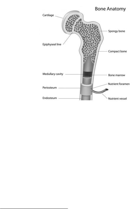
Figure 130: This figure illustrates the principle anatomical features of bone.
The bone itself is a composite material made up of a mix of living and dead cells embedded in a mineralized organic matrix. It has significant tensor structure – looking somewhat like a random honeycomb structure in cross section but with a laminated microstructure along the length of the bone. Its anatomy is illustrated in figure 130.
Bone is layered from the outside in. The very outer hard layer of a bone is called is periosteum199. In between is compact bone, or osteon that gives bone much of its strength. Nutrients flow into living bone tissue through holes in the bone called foramen, and are distributed up and down through the osteon through haversian canals (not shown) that are basically tubes through the bone for blood vessels that run along the bone’s length to perfuse it. The periosteum and osteon make up roughly 80% of the mass of a typical long bone.
Inside the osteon is softer inner bone called endosteum200. The inner bone is made up of a mix of di erent kinds of bone and other tissue that include spongy bone called trabeculae and bone marrow (where blood cells are stored and formed). It has only 20% of the bone’s mass, but 90% of the bone’s surface area. Much of the spongy bone material is filled with blood, to the point where a good way to characterize the di erence between the osteon and the trabeculae is that in the former, bone surrounds blood but in the latter, blood surrounds bone.
199Latin for “outer bone”. But it sounds much cooler in Latin, doesn’t it?
200Latin for – wait for it – “inner bone”.
424 |
Week 9: Oscillations |
The bone matrix itself is made up of a mix of inorganic and organic parts. The inorganic part is formed mostly of calcium hydroxylapatite (a kind of calcium phosphate that is quite rigid). The organic part is collagen, a protein that gives bone its toughness and elasticity in much the same way that tough steels are often a mix of soft iron and hard cementite particles, with the latter contributing hardness and compressive/extensive strength, the latter reducing the brittleness that often accompanies hardness and giving it a broader range of linear response elasticity.
There are two types of microscopically distinct bone. Woven bone has collagen fibers mixed haphazardly with the inorganic matrix, and is mechanically weak. Lamellar bone has a regular parallel alignment of collagen fibers into sheets (lamellae) that is mechanically strong. The latter give the osteon a laminar/layered structure aligned with the bone axis. Woven bone is an early developmental state of lamellar bone, seen in fetuses developing bones and in adults as the initial soft bone that forms in a healing fracture. It serves as a sort of template for the replacement/formation of lamellar bone.
Bones are typically connected together with surface layers of cartilage at the joints, augmented by tough connective tissue and tendons smoothly integrated into muscles that permit mobile bones to be articulated at the joints. Together, they make an impressive mechanical structure capable of an extraordinary range of motions and activities while still supporting and protecting softer tissue of our organs and circulatory system. Pretty cool!
Bone is quite strong. It fractures under compression at a stress of around 170 MPa in typical human bones, but has a smaller fracture stress under tension at 120 MPa and is relatively ¡I¿easy¡/i¿ to fracture with shear stresses of around 52 MPa. This is why it is “easy” (and common!) to break bones with shear stresses, less common to break them from naked compression or tension – typically other parts of the skeletal structure – tendons or cartilage in the joints – fail before the actual bone does in these situations.
Bone is basically brittle and easy to chip, but does have a significant degree of compressive, tensile, or shear elasticity (represented by e.g. Young’s modulus in the linear regime) contributed primarily by collagen in the bone tissue. Younger humans still have relatively elastic bones; as one ages one’s bones become first harder and tougher, and then (as repair mechanisms break down with age) weaker and more brittle.
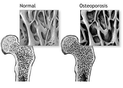
Figure 131: Illustration of the alteration of bone tissue accompanying osteoporosis.
Figure 131 above shows the changes in bone associated with osteoporosis, the gradual thinning
Week 9: Oscillations |
425 |
of the bone matrix as the skeleton starts to decalcify. This process is associated with age, especially in post-menopausal women, but it can also occur in association with e.g. corticosteroid therapy, cancer, or other diseases or conditions such as Paget’s disease in younger adults.
This process significantly weakens the bones of those a icted to the point where the static shear stresses associated with muscular articulation (for example, standing up) can break bones. A young person might fall and break their hip where a person with really significant osteoporosis can actually break their hip (from the stress of standing) and then fall. This is not a medical textbook and should not be treated as an authoritative guide to the practice of medicine (but rather, as a basis for understanding what one might by trying to learn in a directed study of medicine), but with that said, osteoporosis can be treated to some extent by things like hormone replacement therapy in women (it seems to go with the reduction of estrogen that occurs in menopause), calcium supplementation to help slow the loss of calcium, and certain drugs such as Fosamax (Alendronate) that reduce calcium loss and increase bone density (but that have risks and side e ects).
Example 9.6.1: Scaling of Bones with Animal Size
An interesting biological example of scaling laws in physics – and the reason I emphasize the dependence of many physically or physiologically interesting quantities on length and/or area – can be seen in the scaling of animal bones with the size of the animal201 . Let us consider this.
We have seen above that the scaling of the “spring constant” of a given material that governs its change in length or its transverse displacement under compression, tension, or shear is:
ke = |
XA |
(890) |
|
L |
|||
|
|
where X is the relevant (compression, tension, shear) modulus. Bone strength, including the point where the bone fractures under stresses of these sorts, might very reasonably be expected to be proportional to this constant and to scale similarly.
The leg bones of a four-legged animal have to be able to support the weight of that animal under compressive stress. This enables us to make the following scaling argument:
•In general, the weight of any animal is roughly proportional to its volume. Most animals are mostly made of water, and have a density close to that of water, so the volume of the animal times the density of water is a decent approximate guess of what its weight should be.
•In general, the volume of an animal (and hence its weight) is proportional to any characteristic length scale that describes the animal cubed. Obviously this won’t work well if one compares a snake, with one very long length and two very short lengths, to a comparatively round hippopotamus, but it won’t be crazy comparing mice to dogs to horses to elephants that all have reasonably similar body proportions. We’ll choose the animal height.
•The leg bones of the animal have a strength proportional to the cross-sectional area.
We would like to be able to estimate the thickness of an animal’s bone it’s known height and from a knowledge of the thickness of one kind of a “reference” animal’s bone and its height.
Our argument then is: The volume, and hence the weight, of an animal increases like the cube of its characteristic length (e.g. its height H). The strength of its bones that must support this weight goes like the square of the diameter D of those bones. Therefore:
H3 = CD2 |
(891) |
201Wikipedia: http://www.wikipedia.org/wiki/On Being the Right Size. This and many other related arguments were collected by J. B. S. Haldane in an article titled On Being the Right Size, published in 1926. Collectively they are referred to as the Haldane Principle. However, the original idea (and 3/2 scaling law discussed below) is due to none other than Galileo Galilei!
426 |
|
|
Week 9: Oscillations |
where C is some constant of proportionality. Solving for D(H) we get: |
|
||
1 |
H3/2 |
|
|
D = √ |
|
(892) |
|
C |
This simple equation is approximately satisfied, although not exactly as given because our model for bones breaking does not reflect shear-driven ”buckling” and a related need for muscle to scale, for mammals ranging from small rodents through the mighty elephant. Bone thickness does indeed increase nonlinearly with respect to body size.