x

H

R?

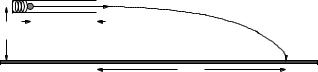
Figure 36: A simple spring gun is fired horizontally a height H above the ground. Compute its range R.

So our first chore then is to compute the work done by the spring that is initially compressed a distance x, and use that in turn to find the speed of the bullet leaving the barrel.

As you can see, this was pretty easy. It is also a result that we can get no other way, so far, because we don’t know how to solve the equations of motion for the mass on the spring to find x(t), solve for t, find v(t), substitute to find v and so on. If we hadn’t derived the WKE theorem for non-constant forces we’d be screwed!

The rest should be familiar. Given this speed (in the x-direction), find the range from Newton’s Laws:

or ax = 0, ay = −g, v0x = vf , v0y = 0, x0 = 0, y0 = H. Solving as usual, we find:

where you can either fill in the details for yourself or look back at your homework. Or get help, of course. If you can’t do this second part on your own at this point, you probably should get help, seriously.

3.3: Conservative Forces: Potential Energy

We have now seen two kinds of forces in action. One kind is like gravity. The work done on a particle by gravity doesn’t depend on the path taken through the gravitational field – it only depends on the relative height of the two endpoints. The other kind is like friction. Friction not only depends on the path a particle takes, it is usually negative work; typically friction turns macroscopic mechanical energy into “heat”, which can crudely be thought of an internal microscopic mechanical energy that can no longer easily be turned back into macroscopic mechanical energy. A proper discussion of

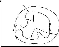
Figure 37: The work done going around an arbitrary loop by a conservative force is zero. This ensures that the work done going between two points is independent of the path taken, its defining characteristic.

heat is beyond the scope of this course, but we will remark further on this below when we discuss non-conservative forces.

We define a conservative force to be one such that the work done by the force as you move a point mass from point ~x1 to point ~x2 is independent of the path used to move between the points:

In this case (only), the work done going around an arbitrary closed path (starting and ending on the same point) will be identically zero!

I

~ ~

Wloop = F · dl = 0 (275)

C

This is illustrated in figure 37. Note that the two paths from ~x1 to ~x2 combine to form a closed loop C, where the work done going forward along one path is undone coming back along the other.

Since the work done moving a mass m from an arbitrary starting point to any point in space is the same independent of the path, we can assign each point in space a numerical value: the work done by us on mass m, against the conservative force, to reach it. This is the negative of the work done by the force. We do it with this sign for reasons that will become clear in a moment. We call

~

this function the potential energy of the mass m associated with the conservative forceF :

Note Well: that only one limit of integration depends on x; the other depends on where you choose to make the potential energy zero. This is a free choice. No physical result that can be measured or observed can uniquely depend on where you choose the potential energy to be zero. Let’s understand this.

3.3.1: Force from Potential Energy

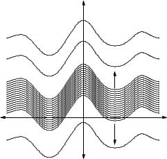
Figure 38: A tiny subset of the infinite number of possible U (x) functions that might lead to the same physical force Fx(x). One of these is highlighted by means of a thick line, but the only thing that might make it “preferred” is whether or not it makes solving any given problem a bit easier.

That is, the force is the slope of the potential energy function. This is actually a rather profound result and relationship.

Consider the set of transformations that leave the slope of a function invariant. One of them is quite obvious – adding a positive or negative constant to U (x) as portrayed in figure 38 does not a ect its slope with respect to x, it just moves the whole function up or down on the U -axis. That means that all of this infinite set of candidate potential energies that di er by only a constant overall energy lead to the same force!

That’s good, as force is something we can often measure, even “at a point” (without necessarily moving the object), but potential energy is not. To measure the work done by a conservative force on an object (and hence measure the change in the potential energy) we have to permit the force to move the object from one place to another and measure the change in its speed, hence its kinetic energy. We only measure a change, though – we cannot directly measure the absolute magnitude of the potential energy, any more than we can point to an object and say that the work of that object is zero Joules, or ten Joules, or whatever. We can talk about the amount of work done moving the object from here to there but objects do not possess “work” as an attribute, and potential energy is just a convenient renaming of the work, at least so far.

I cannot, then, tell you precisely what the near-Earth gravitational potential energy of a 1 kilogram mass sitting on a table is, not even if you tell me exactly where the table and the mass are in some sort of Universal coordinate system (where if the latter exists, as now seems dubious given our discussion of inertial frames and so on, we have yet to find it). There are literally an infinity of possible answers that will all equally well predict the outcome of any physical experiment involving near-Earth gravity acting on the mass, because they all lead to the same force acting on the object.

In more than one dimesion we have to use a bit of vector calculus to write this same result per component:

It’s a bit more work than we can do in this course to prove it, but the result one gets by “dividing

~

through but dℓ” in this case is:

which is basically the one dimensional result written above, per component. If you are a physics or math major (or have had or are in multivariate calculus) this last form should be studied until it makes sense, but everybody should know the first form (per component) and should be able to see that it should reasonably hold (subject to working out some more math than you may yet know) for all coordinate directions. Note that non-physics majors won’t (in my classes) be held responsible for knowing this vector calculus form, but everybody should understand the concept underlying it. We’ll discuss this a bit further below, after we have learned about the total mechanical energy.

So much for the definition of a conservative force, its potential energy, and how to get the force back from the potential energy and our freedom to choose add a constant energy to the potential energy and still get the same answers to all physics problems83 we had a perfectly good theorem, the Work-Kinetic Energy Theorem Why do we bother inventing all of this complication, conservative forces, potential energies? What was wrong with plain old work?

Well, for one thing, since the work done by conservative forces is independent of the path taken by definition, we can do the work integrals once and for all for the well-known conservative forces, stick a minus sign in front of them, and have a set of well-known potential energy functions that are generally even simpler and more useful. In fact, since one can easily di erentiate the potential energy function to recover the force, one can in fact forget thinking in terms of the force altogether and formulate all of physics in terms of energies and potential energy functions!

In this class, we won’t go to this extreme – we will simply learn both the forces and the associated potential energy functions where appropriate (there aren’t that many, this isn’t like learning all of organic chemistry’s reaction pathways or the like), deriving the second from the first as we go, but in future courses taken by a physics major, a chemistry major, a math major it is quite likely that you will relearn even classical mechanics in terms of the Lagrangian84 or Hamiltonian85 formulation, both of which are fundamentally energy-based, and quantum physics is almost entirely derived and understood in terms of Hamiltonians.

For now let’s see how life is made a bit simpler by deriving general forms for the potential energy functions for near-Earth gravity and masses on springs, both of which will be very useful indeed to us in the weeks to come.

3.3.2: Potential Energy Function for Near-Earth Gravity

The potential energy of an object experiencing a near-Earth gravitational force is either:

Z y

Ug (y) = − (−mg)dy′ = mgy (282)

0

where we have e ectively set the zero of the potential energy to be “ground level”, at least if we put the y-coordinate origin at the ground. Of course, we don’t really need to do this – we might well want the zero to be at the top of a table over the ground, or the top of a cli well above that, and we are free to do so. More generally, we can write the gravitational potential energy as the indefinite

integral:

Z

where U0 is an arbitrary constant that sets the zero of gravitational potential energy. For example, suppose we did want the potential energy to be zero at the top of a cli of height H, but for one

83Wikipedia: http://www.wikipedia.org/wiki/Gauge Theory. For students intending to continue with more physics, this is perhaps your first example of an idea called Gauge freedom – the invariance of things like energy under certain sets of coordinate transformations and the implications (like invariance of a measured force) of the symmetry groups of those transformations – which turns out to be very important indeed in future courses. And if this sounds strangely like I’m speaking Martian to you or talking about your freedom to choose a 12 gauge shotgun instead of a 20 gauge shotgun – gauge freedom indeed – well, don’t worry about it...

84Wikipedia: http://www.wikipedia.org/wiki/Lagrangian.

85Wikipedia: http://www.wikipedia.org/wiki/Hamiltonian.