368 Week 8: Fluids

the bottom as it moves forward to become the second surface (darkly shaded) drawn at the top and the bottom, e ecting this net transfer of mass m.

The force F1 exerted to the right on this block of fluid at the bottom is just F1 = P1A1; the force F2 exerted to the left on this block of fluid at the top is similarly F2 = P2A2. The work done by the pressure acting over a distance d at the bottom is W1 = P1A1d, at the top it is W2 = −P2A2D. The total work is equal to the total change in mechanical energy of the chunk m:

There, that wasn’t so di cult, was it? This lovely result is known as Bernoulli’s Principle (or the Bernoulli fluid equation). It contains pretty much everything we’ve done so far except conservation of flow (which is a distinct result, for all that we used it in the derivation) and Archimedes’ Principle.

For example, if v1 = v2 = 0, it describes a static fluid:

and if we change variables to make z (depth) −y (negative height) we get the familiar:

for a static incompressible fluid. It also not only tells us that pressure drops where fluid velocity increases, it tells us how much the pressure drops when it increases, allowing for things like the fluid flowing up or downhill at the same time! Very powerful formula, and all it is is the Work-Mechanical Energy theorem (per unit volume, as we divided out V in the derivation, note well) applied to the fluid!

Example 8.4.1: Emptying the Iced Tea

8.4.3: Fluid Viscosity and Resistance

In the discussion above, we have consistently ignored viscosity and drag, which behave like “friction”, exerting a force parallel to the confining walls of the pipe in the opposite direction to the relative motion of fluid and pipe. In laminar flow, a layer of the fluid “sticks” to the wall and does not move, and the viscosity of the fluid describes the way shear velocity builds up as one goes from the wall of the pipe (velocity zero) to the center of the pipe (maximum velocity). If the fluid is “thick and sticky” (has a large viscosity), fluid in the middle is still experiencing significant backwards force slowing it down, transmitted from the walls to the fluid there. If the fluid is thin and slippery (low visocosity) then fluid even a short distance away from the wall is moving rapidly even thought the fluid “on” the wall itself isn’t moving.

In the absence of any driving force, this drag force will bring fluid flowing in a pipe to rest quite rapidly. To keep it moving, then, requires the continuous application of some driving force. This force, as we shall see, has to maintain a pressure gradient that pushes the fluid through the pipe

from high pressure to low pressure just enough to overcome drag/friction and keep the fluid flowing at a constant speed.

To correctly derive all of this, even for the simplest of geometries, is beyond the scope of this course. It isn’t horribly di cult for a circular pipe, but it requires a treatment of shear stress and viscosity for laminar flow and we don’t yet know what shear stress is. Also, the algebra is a bit involved.

Instead I’m going to invoke my instructor’s privilege (again, but this is pretty close tot he last time) to give you an important result, one that I’d like you to learn even though I do not derive it. I only do this two or three times in this course, and this is, sadly, one of them. To make up for it I will wave my hands and squawk a bit out the result instead, so that you at least conceptually understand where the result comes from and how things scale.

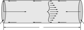
In figure 114 a circular pipe is carrying a fluid with viscosity µ from left to right at a constant speed. Once again, this is a sort of dynamic equilibrium; the net force on the fluid in the pipe segment shown must be zero for the speed of the fluid through it to be maintained unabated during the flow.

The fluid is in contact with and interacts with the walls of the pipe, creating a thin layer of fluid at least a few atoms thick that are “at rest”, stuck to the pipe. As fluid is pushed through the pipe, this layer at rest interacts with and exerts an opposing force on the layer moving just above it via the viscosity of the fluid. This layer in turn interacts with and slows the layer above it and so on right up to the center of the pipe, where the fluid flows most rapidly. The fluid flow thus forms cylindrical layers of constant speed, where the speed increases more or less smoothly from zero where it is contact with the pipe to a peak speed in the middle. The layers are the laminae of laminar flow.

Figure 114: A circular pipe with friction carrying a fluid with viscosity – in other words, a “ real pipe”. This can be a model for everything from household plumbing to the blood vessels of the human circulatory system, within reason.

The interaction of the surface layer with the fluid, redistributed to the whole fluid via the viscosity, exerts a net opposing force on the fluid as it moves through the pipe. In order for the average speed of the fluid to continue, an outside force must act on it with an equal and opposite force. The only available source of this force in the figure is obviously the fluid pressure; if it is larger on the left than on the right (as shown) it will exert a net force on the fluid in between that can balance the drag force exerted by the walls.

The forces at the ends are F1 = P1A, F2 = P2A. The net force acting on the fluid mass is thus:

All things being equal, we expect the flow rate to increase linearly with v, and for laminar flow, the drag force is proportional to v. Therefore we expect that:

We can then divide out the area and write:

Since we cannot derive the constant of proportionality in this expression without doing Evil Math Magic158 we’ll save putting the constants of proportionality in until the end, but we can give what’s called a “hand waving argument” and look at how we expect P to scale with the variables that describe the problem. Hand-waving arguments are actually very important in physics, as we can often use a mix of intuition and dimensional analysis and scaling to guess the right form of a relation to a remarkably accurate degree.

Suppose we had two identical segments of pipe, one right after the other, carrying the same fluid flow. The first pipe needs a drop of P in order to maintain flow I; so does the second. When we put one right after the other, then, we expect the total pressure di erence required to overcome drag to be twice P . From this, we expect the drag force to scale linearly with the length of the pipe; if the pipe is twice as long we need twice the pressure di erence to maintain flow, half as long we need half the pressure di erence. This means that we expect an L (to the first power) on the top in the equation for P .

Next, we expect P (for constant I) to increase monotonically with the viscosity µ. Since the viscosity increases the stickiness and distance the static layer’s reaction force is extended into the fluid, we can’t easily imagine any circumstances where the pressure required to push treacle through a pipe would be less than the pressure required to push plain water. Unfortunately there are an infinite number of monotonically increasing functions of µ available, all heuristically possible. Fortunately all of them have a Taylor Series expansion with a leading linear term so it seems reasonable to at least try a linear dependence (which turns out to work well physically throughout the laminar flow region right up to where the Reynolds number for the fluid flow indicates a – yes, highly nonlinear – transition from laminar/linear drag to nonlinear drag, as we would expect from our Week 2 discussion on drag). So we’ll stick an µ on top.

Finally, suppose we have two identical pipe segments, each carrying identical flow I of identical fluids across identical lengths L through identical cross-sectional areas with identical force di erence F (Note well: not P ) across the pipes. If we put them side by side, two pipes carry twice as much fluid – we already know that the flow itself scales with the area of the aperture. We therefore expect the flow itself to double if we double the cross-sectional area at constant force di erence, and hence we expect to need half the force to maintain the same flow if we double the area at the same force di erence. This puts another factor of A, the cross-sectional area of the pipe, on the bottom.

All that’s missing is the constant of proportionality. Note that all of our scaling arguments above would work for almost any cross-sectional shape of pipe – there is nothing about them that absolutely requires circular pipes. We rather expect that the constant of proportionality for di erent shapes would be di erent, and we have no idea how to compute one – it seems as though it would depend on integrals of some sort over the area or around the perimeter of the pipe but we’d have to have a better model for the relationship between viscosity and force to be able to formulate them.

This, and this only I am going to just give you the answer on. The correct constant of propor-

158Defined as anything requiring more than a page of algebra, serious partial derivatives, and concepts we haven’t

covered yet...

where I have introduced the resistance of the pipe to flow:

Equation 764 is know as Poiseuille’s Law and is a key relation for physicians and plumbers to know because it describes both flow of water in pipes and the flow of blood in blood vessels wherever the flow is slow enough that it is laminar and not turbulent (which is actually “mostly”, so that the expression is useful ).

Before moving on, let me note that P = IR is the fluid-flow version of a named formula in electricity and magnetism (from next semester): Ohm’s Law. The hand-waving “derivation” of Ohm’s Law there will be very similar, with all of the scaling worked out using intuition but a final constant of proportionality that includes the details of the resistive material turned at the last minute into a parameter called the resistivity159.

8.4.4: A Brief Note on Turbulence

You will not be responsible for the formulas or numbers in this section, but you should be conceptually aware of the phenomenon of the “onset of turbulence” in fluid flow. The velocity of the flow in a circular pipe (and other parameters such as µ and r) can be transformed into a general dimensionless parameter called the Reynolds Number Re160 . The Reynolds number for a circular pipe is:

where D = 2r is the hydraulic diameter161 , which in the case of a circular pipe is the actual diameter. One can (as you can see) express Poiseuille’s Law in terms of the Reynolds number, although there is no particular benefit to doing so.

The one thing the Reynolds number does for us is that it serves as a marker for the transition to turbulent flow. For Re < 2300 flow in a circular pipe is laminar and all of the relations above hold. Turbulent flow occurs for Re > 4000. In between is the region known as the onset of turbulence, where the resistance of the pipe depends on flow in a very nonlinear fashion, and among other things dramatically increases with the Reynolds number. As we will see in a moment (in an example) this means that the partial occlusion of blood vessels can have a profound e ect on the human circulatory system.

At this point you should understand fluid statics and dynamics quite well, armed both with equations such as the Bernoulli Equation that describe idealized fluid dynamics and statics as well as with conceptual (but possibly quantitative) ideas such Pascal’s Principle or Archimedes’ principle as the relationship between pressure di erences, flow, and the geometric factors that contribute to resistance. Let’s put some of this nascent understanding to the test by looking over and analyzing the human circulatory system.