Figure 23: A simple object falling through a fluid experiences a drag force of Fd = −blv. In the figure above m = 100 kg, g = 9.8 m/sec2, and bl = 19.6, so that terminal velocity is 50 m/sec. Compare this figure to figure 25 below and note that it takes a relatively longer time to reach the same terminal velocity for an object of the same mass. Note also that the bl that permits the terminal velocities to be the same is much larger than bt!

2.2.4: Advanced: Solution to Equations of Motion for Turbulent Drag

Turbulent drag is set up exactly the same way that Stokes’ drag is We suppose an object is dropped from rest and almost immediately converts to a turbulent drag force. This can easily happen because it has a blu shape or an irregular surface together with a large coupling between that surface and the surrounding fluid (such as one might see in the following example, with a furry, flu y ram).

The one “catch” is that the integral you have to do is a bit di cult for most physics students to do, unless they were really good at calculus. We will use a special method to solve this integral in the example below, one that I commend to all students when confronted by problems of this sort.

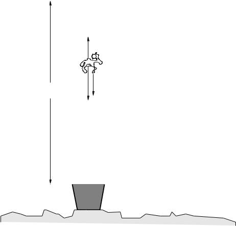
Example 2.2.3: Dropping the Ram

The UNC ram, a wooly beast of mass Mram is carried by some naughty (but intellectually curious) Duke students up in a helicopter to a height H and is thrown out. On the ground below a student armed with a radar gun measures and records the velocity of the ram as it plummets toward the vat of dark blue paint below63. Assume that the flu y, cute little ram experiences a turbulent drag force on the way down of −btv2 in the direction shown.

In terms of these quantities (and things like g):

a)Describe qualitatively what you expect to see in the measurements recorded by the student (v(t)).

b)What is the actual algebraic solution v(t) in terms of the givens.

c)Approximately how fast is the fat, furry creature going when it splashes into the paint, more or less permanently dying it Duke Blue, if it has a mass of 100 kg and is dropped from a height

63Note well: No real sheep are harmed in this physics problem – this actual experiment is only conducted with soft,

cuddly, stu ed sheep...

mathematicians (and perhaps some not so famous ones) worked all of this sort of thing out. Once upon a time you and I probably worked out how to solve this in a calculus class. But we forgot (at least I did – I took integral calculus in the spring of 1973, almost forty years ago as I write this). So what the heck, look it up!

Now you know what those rarely used buttons on your calculator are for. We substitute x− > v, p

a → mg/b, multiply out the mg/b and then take the hyperbolic tangent of both sides and then p

multiply by mg/b again to get the following result for the speed of descent as a function of time:

rÃr !

This solution is plotted for you as a function of time in figure 25 below.

Figure 25: A simple object falling through a fluid experiences a drag force of Fd = −btv2. In the figure above (generated using the numbers given in the ram example), m = 100 kg, g = 9.8 m/sec2, and bt = 0.392, so that terminal velocity is 50 m/sec. Note that the initial acceleration is g, but

that after falling around 14 seconds the object is travelling at a speed very close to terminal velocity.

p

√

Since even without drag forces it takes 2H/g ≈ 200 ≈ 14 seconds to fall 1000 meters, it is almost certain that the ram will be travelling at the terminal velocity of 50 m/sec as it hits the paint!

Clearly this is a lot of algebra, but that’s realistic (or more so than Stokes’ drag for most problems). It’s just the way nature really is, tough luck and all that. If we want any consolation, at least we didn’t have to try to integrate over the transition between Stokes’ drag and full-blown turbulent drag for the specific shape of a furry ram being dropped from underneath a helicopter (that no doubt has made the air it falls through initially both turbulent and beset by a substantial downdraft).

Real physics is often not terribly easy to compute, but the good thing is that it is still easy enough to understand. Even if we have a hard time answering question b) above, we should all be able to understand and draw a qualitative picture for a) and we should really even be able to guess that the ram is moving at or near terminal velocity by the time it has fallen 1000 meters.

2.3: Inertial Reference Frames – the Galilean Transformation

We have already spoken about coordinate systems, or “frames”, that we need to imagine when we create the mental map between a physics problem in the abstract and the supposed reality that it describes. One immediate problem we face is that there are many frames we might choose to solve a problem in, but that our choice of frames isn’t completely arbitrary. We need to reason out how much freedom we have, so that we can use that freedom to make a “good choice” and select a frame that makes the problem relatively simple.

Students that go on in physics will learn that there is more to this process than meets the eye – the symmetries of frames that preserve certain quantities actually leads us to an understanding of conserved quantities and restricts acceptable physical theories in certain key ways. But even students with no particular interest in relativity theory or quantum theory or advanced classical mechanics (where all of this is developed) have to understand the ideas developed in this section, simply to be able to solve problems e ciently.