

- •Preface
- •Textbook Layout and Design
- •Preliminaries
- •See, Do, Teach
- •Other Conditions for Learning
- •Your Brain and Learning
- •The Method of Three Passes
- •Mathematics
- •Summary
- •Homework for Week 0
- •Summary
- •1.1: Introduction: A Bit of History and Philosophy
- •1.2: Dynamics
- •1.3: Coordinates
- •1.5: Forces
- •1.5.1: The Forces of Nature
- •1.5.2: Force Rules
- •Example 1.6.1: Spring and Mass in Static Force Equilibrium
- •1.7: Simple Motion in One Dimension
- •Example 1.7.1: A Mass Falling from Height H
- •Example 1.7.2: A Constant Force in One Dimension
- •1.7.1: Solving Problems with More Than One Object
- •Example 1.7.4: Braking for Bikes, or Just Breaking Bikes?
- •1.8: Motion in Two Dimensions
- •Example 1.8.1: Trajectory of a Cannonball
- •1.8.2: The Inclined Plane
- •Example 1.8.2: The Inclined Plane
- •1.9: Circular Motion
- •1.9.1: Tangential Velocity
- •1.9.2: Centripetal Acceleration
- •Example 1.9.1: Ball on a String
- •Example 1.9.2: Tether Ball/Conic Pendulum
- •1.9.3: Tangential Acceleration
- •Homework for Week 1
- •Summary
- •2.1: Friction
- •Example 2.1.1: Inclined Plane of Length L with Friction
- •Example 2.1.3: Find The Minimum No-Skid Braking Distance for a Car
- •Example 2.1.4: Car Rounding a Banked Curve with Friction
- •2.2: Drag Forces
- •2.2.1: Stokes, or Laminar Drag
- •2.2.2: Rayleigh, or Turbulent Drag
- •2.2.3: Terminal velocity
- •Example 2.2.1: Falling From a Plane and Surviving
- •2.2.4: Advanced: Solution to Equations of Motion for Turbulent Drag
- •Example 2.2.3: Dropping the Ram
- •2.3.1: Time
- •2.3.2: Space
- •2.4.1: Identifying Inertial Frames
- •Example 2.4.1: Weight in an Elevator
- •Example 2.4.2: Pendulum in a Boxcar
- •2.4.2: Advanced: General Relativity and Accelerating Frames
- •2.5: Just For Fun: Hurricanes
- •Homework for Week 2
- •Week 3: Work and Energy
- •Summary
- •3.1: Work and Kinetic Energy
- •3.1.1: Units of Work and Energy
- •3.1.2: Kinetic Energy
- •3.2: The Work-Kinetic Energy Theorem
- •3.2.1: Derivation I: Rectangle Approximation Summation
- •3.2.2: Derivation II: Calculus-y (Chain Rule) Derivation
- •Example 3.2.1: Pulling a Block
- •Example 3.2.2: Range of a Spring Gun
- •3.3: Conservative Forces: Potential Energy
- •3.3.1: Force from Potential Energy
- •3.3.2: Potential Energy Function for Near-Earth Gravity
- •3.3.3: Springs
- •3.4: Conservation of Mechanical Energy
- •3.4.1: Force, Potential Energy, and Total Mechanical Energy
- •Example 3.4.1: Falling Ball Reprise
- •Example 3.4.2: Block Sliding Down Frictionless Incline Reprise
- •Example 3.4.3: A Simple Pendulum
- •Example 3.4.4: Looping the Loop
- •3.5: Generalized Work-Mechanical Energy Theorem
- •Example 3.5.1: Block Sliding Down a Rough Incline
- •Example 3.5.2: A Spring and Rough Incline
- •3.5.1: Heat and Conservation of Energy
- •3.6: Power
- •Example 3.6.1: Rocket Power
- •3.7: Equilibrium
- •3.7.1: Energy Diagrams: Turning Points and Forbidden Regions
- •Homework for Week 3
- •Summary
- •4.1: Systems of Particles
- •Example 4.1.1: Center of Mass of a Few Discrete Particles
- •4.1.2: Coarse Graining: Continuous Mass Distributions
- •Example 4.1.2: Center of Mass of a Continuous Rod
- •Example 4.1.3: Center of mass of a circular wedge
- •4.2: Momentum
- •4.2.1: The Law of Conservation of Momentum
- •4.3: Impulse
- •Example 4.3.1: Average Force Driving a Golf Ball
- •Example 4.3.2: Force, Impulse and Momentum for Windshield and Bug
- •4.3.1: The Impulse Approximation
- •4.3.2: Impulse, Fluids, and Pressure
- •4.4: Center of Mass Reference Frame
- •4.5: Collisions
- •4.5.1: Momentum Conservation in the Impulse Approximation
- •4.5.2: Elastic Collisions
- •4.5.3: Fully Inelastic Collisions
- •4.5.4: Partially Inelastic Collisions
- •4.6: 1-D Elastic Collisions
- •4.6.1: The Relative Velocity Approach
- •4.6.2: 1D Elastic Collision in the Center of Mass Frame
- •4.7: Elastic Collisions in 2-3 Dimensions
- •4.8: Inelastic Collisions
- •Example 4.8.1: One-dimensional Fully Inelastic Collision (only)
- •Example 4.8.2: Ballistic Pendulum
- •Example 4.8.3: Partially Inelastic Collision
- •4.9: Kinetic Energy in the CM Frame
- •Homework for Week 4
- •Summary
- •5.1: Rotational Coordinates in One Dimension
- •5.2.1: The r-dependence of Torque
- •5.2.2: Summing the Moment of Inertia
- •5.3: The Moment of Inertia
- •Example 5.3.1: The Moment of Inertia of a Rod Pivoted at One End
- •5.3.1: Moment of Inertia of a General Rigid Body
- •Example 5.3.2: Moment of Inertia of a Ring
- •Example 5.3.3: Moment of Inertia of a Disk
- •5.3.2: Table of Useful Moments of Inertia
- •5.4: Torque as a Cross Product
- •Example 5.4.1: Rolling the Spool
- •5.5: Torque and the Center of Gravity
- •Example 5.5.1: The Angular Acceleration of a Hanging Rod
- •Example 5.6.1: A Disk Rolling Down an Incline
- •5.7: Rotational Work and Energy
- •5.7.1: Work Done on a Rigid Object
- •5.7.2: The Rolling Constraint and Work
- •Example 5.7.2: Unrolling Spool
- •Example 5.7.3: A Rolling Ball Loops-the-Loop
- •5.8: The Parallel Axis Theorem
- •Example 5.8.1: Moon Around Earth, Earth Around Sun
- •Example 5.8.2: Moment of Inertia of a Hoop Pivoted on One Side
- •5.9: Perpendicular Axis Theorem
- •Example 5.9.1: Moment of Inertia of Hoop for Planar Axis
- •Homework for Week 5
- •Summary
- •6.1: Vector Torque
- •6.2: Total Torque
- •6.2.1: The Law of Conservation of Angular Momentum
- •Example 6.3.1: Angular Momentum of a Point Mass Moving in a Circle
- •Example 6.3.2: Angular Momentum of a Rod Swinging in a Circle
- •Example 6.3.3: Angular Momentum of a Rotating Disk
- •Example 6.3.4: Angular Momentum of Rod Sweeping out Cone
- •6.4: Angular Momentum Conservation
- •Example 6.4.1: The Spinning Professor
- •6.4.1: Radial Forces and Angular Momentum Conservation
- •Example 6.4.2: Mass Orbits On a String
- •6.5: Collisions
- •Example 6.5.1: Fully Inelastic Collision of Ball of Putty with a Free Rod
- •Example 6.5.2: Fully Inelastic Collision of Ball of Putty with Pivoted Rod
- •6.5.1: More General Collisions
- •Example 6.6.1: Rotating Your Tires
- •6.7: Precession of a Top
- •Homework for Week 6
- •Week 7: Statics
- •Statics Summary
- •7.1: Conditions for Static Equilibrium
- •7.2: Static Equilibrium Problems
- •Example 7.2.1: Balancing a See-Saw
- •Example 7.2.2: Two Saw Horses
- •Example 7.2.3: Hanging a Tavern Sign
- •7.2.1: Equilibrium with a Vector Torque
- •Example 7.2.4: Building a Deck
- •7.3: Tipping
- •Example 7.3.1: Tipping Versus Slipping
- •Example 7.3.2: Tipping While Pushing
- •7.4: Force Couples
- •Example 7.4.1: Rolling the Cylinder Over a Step
- •Homework for Week 7
- •Week 8: Fluids
- •Fluids Summary
- •8.1: General Fluid Properties
- •8.1.1: Pressure
- •8.1.2: Density
- •8.1.3: Compressibility
- •8.1.5: Properties Summary
- •Static Fluids
- •8.1.8: Variation of Pressure in Incompressible Fluids
- •Example 8.1.1: Barometers
- •Example 8.1.2: Variation of Oceanic Pressure with Depth
- •8.1.9: Variation of Pressure in Compressible Fluids
- •Example 8.1.3: Variation of Atmospheric Pressure with Height
- •Example 8.2.1: A Hydraulic Lift
- •8.3: Fluid Displacement and Buoyancy
- •Example 8.3.1: Testing the Crown I
- •Example 8.3.2: Testing the Crown II
- •8.4: Fluid Flow
- •8.4.1: Conservation of Flow
- •Example 8.4.1: Emptying the Iced Tea
- •8.4.3: Fluid Viscosity and Resistance
- •8.4.4: A Brief Note on Turbulence
- •8.5: The Human Circulatory System
- •Example 8.5.1: Atherosclerotic Plaque Partially Occludes a Blood Vessel
- •Example 8.5.2: Aneurisms
- •Homework for Week 8
- •Week 9: Oscillations
- •Oscillation Summary
- •9.1: The Simple Harmonic Oscillator
- •9.1.1: The Archetypical Simple Harmonic Oscillator: A Mass on a Spring
- •9.1.2: The Simple Harmonic Oscillator Solution
- •9.1.3: Plotting the Solution: Relations Involving
- •9.1.4: The Energy of a Mass on a Spring
- •9.2: The Pendulum
- •9.2.1: The Physical Pendulum
- •9.3: Damped Oscillation
- •9.3.1: Properties of the Damped Oscillator
- •Example 9.3.1: Car Shock Absorbers
- •9.4: Damped, Driven Oscillation: Resonance
- •9.4.1: Harmonic Driving Forces
- •9.4.2: Solution to Damped, Driven, Simple Harmonic Oscillator
- •9.5: Elastic Properties of Materials
- •9.5.1: Simple Models for Molecular Bonds
- •9.5.2: The Force Constant
- •9.5.3: A Microscopic Picture of a Solid
- •9.5.4: Shear Forces and the Shear Modulus
- •9.5.5: Deformation and Fracture
- •9.6: Human Bone
- •Example 9.6.1: Scaling of Bones with Animal Size
- •Homework for Week 9
- •Week 10: The Wave Equation
- •Wave Summary
- •10.1: Waves
- •10.2: Waves on a String
- •10.3: Solutions to the Wave Equation
- •10.3.1: An Important Property of Waves: Superposition
- •10.3.2: Arbitrary Waveforms Propagating to the Left or Right
- •10.3.3: Harmonic Waveforms Propagating to the Left or Right
- •10.3.4: Stationary Waves
- •10.5: Energy
- •Homework for Week 10
- •Week 11: Sound
- •Sound Summary
- •11.1: Sound Waves in a Fluid
- •11.2: Sound Wave Solutions
- •11.3: Sound Wave Intensity
- •11.3.1: Sound Displacement and Intensity In Terms of Pressure
- •11.3.2: Sound Pressure and Decibels
- •11.4: Doppler Shift
- •11.4.1: Moving Source
- •11.4.2: Moving Receiver
- •11.4.3: Moving Source and Moving Receiver
- •11.5: Standing Waves in Pipes
- •11.5.1: Pipe Closed at Both Ends
- •11.5.2: Pipe Closed at One End
- •11.5.3: Pipe Open at Both Ends
- •11.6: Beats
- •11.7: Interference and Sound Waves
- •Homework for Week 11
- •Week 12: Gravity
- •Gravity Summary
- •12.1: Cosmological Models
- •12.2.1: Ellipses and Conic Sections
- •12.4: The Gravitational Field
- •12.4.1: Spheres, Shells, General Mass Distributions
- •12.5: Gravitational Potential Energy
- •12.6: Energy Diagrams and Orbits
- •12.7: Escape Velocity, Escape Energy
- •Example 12.7.1: How to Cause an Extinction Event
- •Homework for Week 12
240 |
Week 5: Torque and Rotation in One Dimension |
In particular, this equation contains the moment of inertia of a point mass m moving in a circle of radius r:
Ipoint mass = mr2 |
(466) |
This looks like, and of course is, Newton’s Second Law for a rigid rotating system in one dimension, where force is replaced by torque, mass is replaced by moment of inertia, and linear acceleration is replaced by angular acceleration.
Although to us so far this looks just like a trivial algebraic rewrite of something we could have worked with just as easily as the real thing in the s coordinates, it is actually far more general and powerful. To completely understand this, we need to understand two things. One of them is how
~
applying the force F to (for example) the rod at di erent radii rF changes the angular acceleration
~
α. The other is how a force F applied at some radius rF to the massless rod internally redistributes to muliple masses attached to the rod at di erent radii so that all the masses experience the same angular acceleration. These are the subjects of the next two sections.
5.2.1: The R-dependence of Torque
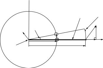
Let’s see how the angular acceleration of this mass will scale with the point of application of the force along the rod, and in the process justify our “inspired decision” to multiply Ft by r in our definition of the torque in the previous section. To accomplish this we need a new figure, one where the massless rigid rod extends out past/through the mass m so it can act as a lever arm on the mass
~
no matter where we choose to apply the force F .
y
rod |
dL = r F dθ |
|
dθ |
F |
|
|
|
|
|
Fp |
m |
Ft |
= F sin( φ) |
|
φ |
|
pivot |
rm |
Fr |
x |
|
|
|
rF
~
Figure 61: The force F is applied to the pivoted rod at an angle φ at the point ~rF with the mass m attached to the rod at radius rm.
This is displayed in figure 61. A massless rod as long or longer than both rm and rF is pivoted at one end so it can swing freely (no friction). The mass m is attached to the rod at the position
~
rm. A force F is applied to the rod at the position ~rF (on the rod) and at an angle φ with respect to the direction of ~rF .
~
Turning this into a suitable angular equation of motion is a bit of a puzzle. The force F is not applied directly to the mass – it is applied to the massless rigid rod which in turn transmits some
~
of the force to the mass. However, the external force F is not the only force acting on the rod!
|
~ |
In the previous example the pivot only exerted a radial force F p = −T , and exerted no tangential |
|
~ |
~ |
force on m at all. We could even compute T (and hence F p) if we knew θ, vt and F from rotational
~
kinematics and some vector geometry. In this case, however, if F exerts a force on the rod that can

Week 5: Torque and Rotation in One Dimension |
241 |
be transmitted to and act tangentially upon the mass m, it rather seems that the unknown pivot
~ ~
force F p can as well, but we don’t know F p!
Alas, without knowing all of the forces that act tangentially on m, we cannot use Newton’s Second Law directly. This motivates us to consider using work and energy to obtain a dynamical principle (basically working the derivation of the WKE theorem backwards) because the pivot does
~
not move and therefore the force F p does no work! Consequently, the fact that we do not yet
~
know F p will not matter!
~
So to work. Let us suppose that the force F is applied to the rod for a time dt, and that during that time the rod rotates through an angle dθ as shown. In this case we can easily find the work
~ |
~ |
dθ. |
done by the force F . The point on the rod where the force F is applied moves a distance dℓ = rF |
||
The work is done only by the tangential component of the force moved through this distance Ft so
that: |
|
|
~ |
~ |
(467) |
dW = F · dℓ = FtrF dθ |
||
The WKE theorem tells us that this work must equal the change in the kinetic energy over that
time: |
¡ |
1 mv2 |
¢ |
|
|
|
|
d |
|
|
|||
FtrF dθ = dK = |
|
2dt t |
dt = mvt dvt |
(468) |
||
We make a few useful substitutions from table 3 above:
FtrF dθ = m |
µrm dt ¶ |
(rmα dt) = mrm2 αdθ |
(469) |
||
|
|
dθ |
|
|
|
and cancel dθ (and reorder a bit) to get: |
|
|
|
|
|
τ = rF Ft = rF F sin(φ) = mrm2 α = Iα |
(470) |
||||
This formally proves that my “guess” of τ = Iα as being the correct form of Newton’s Second Law for this simple rotating rigid body holds up pretty well no matter where we apply the force(s) that make up the torque, as long as we define the torque:
τ = rF Ft = rF F sin(φ) |
(471) |
It is left as an exercise for the student to draw a picture like the one above but involving many
~ |
~ |
acting at ~r2, ..., you get: |
|
independent and arbitrary forces, F 1 |
acting at ~r1, F 2 |
|
|
|
X |
|
|
τtot = |
riFi sin(φi) = mrm2 α = Iα |
(472) |
|
i
for a single point-like mass on the rod at position ~rm. Note well that each φi is the angle between
~
~ri and F i, and you should make the (massless, after all) rod long enough for all of the forces to be able to act on it and also pass through m.
In a bit we will pay attention to the fact that rF sin(φ) is the magnitude of the cross product110
~
of ~rF and F , and that if we assign the direction of the rotation to be parallel to the z-axis of a right handed coordinate system when φ is drawn in the sense shown, we can even make this a vector relation. For the moment, though, we will stick with our simple 1D “scalar” formulation and ask a di erent question: what if we have a more complicated object than a single mass on a pivoted rigid rod that is being driven by a torque (or sum of torques).
The answer is: We have to sum up the object’s total moment of inertia around the pivot axis. Let’s prove this.
110Wikipedia: http://www.wikipedia.org/wiki/Cross Product. Making this a gangbusters good time to go review – or learn – cross products, at least well enough to be able evaluate their magnitude and direction (using the right hand rule).
242 |
Week 5: Torque and Rotation in One Dimension |
5.2.2: Summing the Moment of Inertia
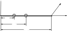
Suppose we have a mass m1 attached to our massless rod pivoted at the origin at the position r1,
~
and a second mass m2 attached at position r2. We will then apply the force F at an angle φ to the (extended) rod at position r as shown in figure 62, and duplicate our reasoning from the last chapter (because we still do not known the unknown force exerted by the pivot, but as long as we consider work we don’t have to.
y 
|
F |
m 1 m 2 |
φ |
r1 |
x |
r2
rF
Figure 62: A single torque τ = rF F sin(φ) is applied to a rod with two masses, m1 at r1 and m2 at r2.
The WKE theorem for this picture is now (note that v1 and v2 are both necessarily tangential):
dW = rF F sin(φ) dθ = τ dθ |
= |
dK = m1v1 dv1 + m2v2dv2 |
so as usual |
||
τ dθ = m1 µr1 dt ¶ (r1α dt) + m2 µr2 dt ¶ |
(r2α dt) |
||||
|
|
|
dθ |
dθ |
|
τ = m1r12α + m2r22α |
|
|
|||
τ |
= |
¡m1r12 + m2r22¢ α = Iα |
|
(473) |
|
where we have now defined |
|
|
|
|
|
|
I = m1r12 + m2r22 |
|
(474) |
||
That is, the total moment of inertia of the two point masses is just the sum of their individual moments of inertia. From the derivation it should be clear that if we added 3,4,...,N point masses along the massless rod the total moment of inertia would just be the sum of their individual moments of inertia.
Indeed, as we add more forces acting at di erent points and directions (in the plane) on the rod and add more masses at di erent points on the rod, everything we did above clearly scales up linearly – we simply have to sum the total torque on the right hand side and sum the total moment of inertia on the left hand side. We therefore conclude that Newton’s Second Law for a system constrained to rotate in (one dimension in a) a plane about a fixed pivot is just:
|
|
|
X |
|
|
|
X |
|
|
|
|
τ |
tot |
= |
r |
F |
sin(φ |
) = |
m r2 |
α = I |
tot |
α |
(475) |
|
|
i |
i |
i |
|
j j |
|
|
|
||
|
|
|
i |
|
|
|
j |
|
|
|
|
So much for discrete forces and discrete masses. However, most rigid bodies that we experience every day are, on a coarse-grained macroscopic scale, made up of a continuous distribution of mass, and instead of a mythical idealized “massless rigid rod” all of this mass is glued together by means of internal forces.
It is pretty clear that our expression τ = Iα will generalize to this case where we will (probably)
replace:
Z
X |
|
I = mj rj2 → r2dm |
(476) |
j
but we will need to do just a teensy bit of work to show that this is true and extract any essential conceptual insight to be found along the way.