

Week 2: Newton’s Laws: Continued |
97 |
a)We will only consider smooth, uniform, nonreactive surfaces of convex, blu objects (like spheres) or streamlined objects (like rockets or arrows) moving through uniform, stationary fluids where we can ignore or treat separately e.g. bouyant forces.
b)We will wrap up all of our ignorance of the shape and cross-sectional area of the object, the density and viscosity of the fluid, and so on in a single number, b. This dimensioned number will only be actually computable for certain particularly “nice” shapes and so on (see the Wikipedia article on drag linked above) but allows us to treat drag relatively simply. We will treat drag in two limits:
c)Low velocity, non-turbulent (streamlined, laminar) motion leads to Stokes’ drag, described
by:
~ |
(140) |
F d = −b~v |
This is the simplest sort of drag – a drag force directly proportional to the velocity of (relative) motion of the object through the fluid and oppositely directed.
d)High velocity, turbulent (high Reynolds number) drag that is described by a quadratic dependence on the relative velocity:
~ |
(141) |
F d = −b|v|~v |
It is still directed opposite to the relative velocity of the object and the fluid but now is proportional to that velocity squared.
e)In between, drag is a bit of a mess – changing over from one from to the other. We will ignore this transitional region where turbulence is appearing and so on, except to note that it is there and you should be aware of it.
•Pseudoforces in an accelerating frame are gravity-like “imaginary” forces we must add to the real forces of nature to get an accurate Newtonian description of motion in a noninertial reference frame. In all cases it is possible to solve Newton’s Laws without recourse to pseudoforces (and this is the general approach we promote in this textbook) but it is useful in a few cases to see how to proceed to solve or formulate a problem using pseudoforces such as “centrifugal force” or “coriolis force” (both arising in a rotating frame) or pseudogravity in a linearly accelerating frame. In all cases if one tries to solve force equations in an accelerating frame, one must modify the actual force being exerted on a mass m in an inertial frame by:
~ |
~ |
(142) |
F accelerating = F intertial − m~aframe |
||
where −m~aframe is the pseudoforce.
This sort of force is easily exemplified – indeed, we’ve already seen such an example in our treatment of apparent weight in an elevator in the first week/chapter.
2.1: Friction
So far, our picture of natural forces as being the cause of the acceleration of mass seems fairly successful. In time it will become second nature to you; you will intuitively connect forces to all changing velocities. However, our description thus far is fairly simplistic – we have massless strings, frictionless tables, drag-free air. That is, we are neglecting certain well-known and important facts or forces that appear in real-world problems in order to concentrate on “ideal” problems that illustrate the methods simply.
It is time to restore some of the complexity to the problems we solve. The first thing we will add is friction.
Experimentally
98 |
Week 2: Newton’s Laws: Continued |
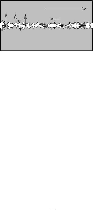
Applied Force F
Normal Force
Frictional Contact Force
Figure 16: A cartoon picture representing two “smooth” surfaces in contact when they are highly magnified. Note the two things that contribute to friction – area in actual contact, which regulates the degree of chemical bonding between the surfaces, and a certain amount of “keyholing” where features in one surface fit into and are physically locked by features in the other.
a)fs ≤ µs |N |. The force exerted by static friction is less than or equal to the coe cient of static friction mus times the magnitude of the normal force exerted on the entire (homogeneous) surface of contact. We will sometimes refer to this maximum possible value of static friction as fsmax = µs |N |. It opposes the component of any (otherwise net) applied force in the plane of the surface to make the total force component parallel to the surface zero as long as it is able to do so (up to this maximum).
b)fk = µk |N |. The force exerted by kinetic friction (produced by two surfaces rubbing against or sliding across each other in motion) is equal to the coe cient of kinetic friction times the magnitude of the normal force exerted on the entire (homogeneous) surface of contact. It opposes the direction of the relative motion of the two surfaces.
c)µk < µs
d)µk is really a function of the speed v (see discussion on drag forces), but for “slow” speeds µk constant and we will idealize it as a constant throughout this book.
e)µs and µk depend on the materials in “smooth” contact, but are independent of contact area.
We can understand this last observation by noting that the frictional force should depend on the pressure (the normal force/area ≡ N/m2) and the area in contact. But then
N |
A = µkN |
|
fk = µkP A = µk A |
(143) |
and we see that the frictional force will depend only on the total force, not the area or pressure separately.
The idealized force rules themselves, we see, are pretty simple: fs ≤ µsN and fk = µkN . Let’s see how to apply them in the context of actual problems.
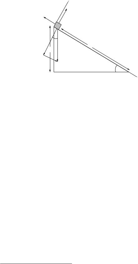
Example 2.1.1: Inclined Plane of Length L with Friction
In figure 17 the problem of a block of mass m released from rest at time t = 0 on a plane of length L inclined at an angle θ relative to horizontal is once again given, this time more realistically, including the e ects of friction. The inclusion of friction enables new questions to be asked that require the
Week 2: Newton’s Laws: Continued |
99 |
y 
fs,k N
m
θ
mg
L
H
θ
x 
Figure 17: Block on inclined plane with both static and dynamic friction. Note that we still use the coordinate system selected in the version of the problem without friction, with the x-axis aligned with the inclined plane.
use of your knowledge of both the properties and the formulas that make up the friction force rules to answer, such as:
a)At what angle θc does the block barely overcome the force of static friction and slide down the incline.?
b)Started at rest from an angle θ > θc (so it definitely slides), how fast will the block be going when it reaches the bottom?
To answer the first question, we note that static friction exerts as much force as necessary to keep the block at rest up to the maximum it can exert, fsmax = µsN . We therefore decompose the known force rules into x and y components, sum them componentwise, write Newton’s Second Law for both vector components and finally use our prior knowledge that the system remains in static force equilibrium to set ax = ay = 0. We get:
X Fx = mg sin(θ) − fs = 0 |
(144) |
(for θ ≤ θc and v(0) = 0) and |
|
X Fy = N − mg cos(θ) = 0 |
(145) |
So far, fs is precisely what it needs to be to prevent motion: |
|
fs = mg sin(θ) |
(146) |
while |
|
N = mg cos(θ) |
(147) |
is true at any angle, moving or not moving, from the Fy equation51. |
|
You can see that as one gradually and gently increases the angle θ, the force that must be exerted by static friction to keep the block in static force equilibrium increases as well. At the same time, the
51Here again is an appeal to experience and intuition – we know that masses placed on inclines under the influence of gravity generally do not “jump up” o of the incline or “sink into” the (solid) incline, so their acceleration in the perpendicular direction is, from sheer common sense, zero. Proving this in terms of microscopic interactions would be absurdly di cult (although in principle possible) but as long as we keep our wits about ourselves we don’t have to!
100 |
Week 2: Newton’s Laws: Continued |
normal force exerted by the plane decreases (and hence the maximum force static friction can exert decreases as well. The critical angle is the angle where these two meet; where fs is as large as it can be such that the block barely doesn’t slide (or barely starts to slide, as you wish – at the boundary the slightest fluctuation in the total force su ces to trigger sliding). To find it, we can substitute fsmax = µsNc where Nc = mg cos(θc) into both equations, so that the first equation becomes:
X Fx = mg sin(θc) − µsmg cos(θc) = 0 |
(148) |
at θc. Solving for θc, we get: |
|
θc = tan−1(µs) |
(149) |
Once it is moving (either at an angle θ > θc or at a smaller angle than this but with the initial condition vx(0) > 0, giving it an initial “push” down the incline) then the block will (probably) accelerate and Newton’s Second Law becomes:
X
Fx = mg sin(θ) − µkmg cos(θ) = max |
(150) |
which we can solve for the constant acceleration of the block down the incline:
ax = g sin(θ) − µkg cos(θ) = g(sin(θ) − µk cos(θ)) |
(151) |
Given ax, it is now straightforward to answer the second question above (or any of a number of others) using the methods exemplified in the first week/chapter. For example, we can integrate twice and find vx(t) and x(t), use the latter to find the time it takes to reach the bottom, and substitute that time into the former to find the speed at the bottom of the incline. Try this on your own, and get help if it isn’t (by now) pretty easy.
Other things you might think about: Suppose that you started the block at the top of an incline at an angle less than θc but at an initial speed vx(0) = v0. In that case, it might well be the case that fk > mg sin(θ) and the block would slide down the incline slowing down. An interesting question might then be: Given the angle, µk, L and v0, does the block come to rest before it reaches the bottom of the incline? Does the answer depend on m or g? Think about how you might formulate and answer this question in terms of the givens.
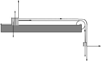
Example 2.1.2: Block Hanging o of a Table
|
+y |
|
N |
m 1 |
+x |
fs,k |
T |
|
m1g |
T |
m2
+y
m 2g
+x
Figure 18: Atwood’s machine, sort of, with one block resting on a table with friction and the other dangling over the side being pulled down by gravity near the Earth’s surface. Note that we should use an “around the corner” coordinate system as shown, since a1 = a2 = a if the string is unstretchable.

Week 2: Newton’s Laws: Continued |
101 |
Suppose a block of mass m1 sits on a table. The coe cients of static and kinetic friction between the block and the table are µs > µk and µk respectively. This block is attached by an “ideal” massless unstretchable string running over an “ideal” massless frictionless pulley to a block of mass m2 hanging o of the table as shown in figure 18. The blocks are released from rest at time t = 0.
Possible questions include:
a)What is the largest that m2 can be before the system starts to move, in terms of the givens and knowns (m1, g, µk, µs...)?
b)Find this largest m2 if m1 = 10 kg and µs = 0.4.
c)Describe the subsequent motion (find a, v(t), the displacement of either block x(t) from its starting position). What is the tension T in the string while they are stationary?
d)Suppose that m2 = 5 kg and µk = 0.3. How fast are the masses moving after m2 has fallen one meter? What is the tension T in the string while they are moving?
Note that this is the first example you have been given with actual numbers. They are there to tempt you to use your calculators to solve the problem. Do not do this! Solve both of these problems algebraically and only at the very end, with the full algebraic answers obtained and dimensionally checked, consider substituting in the numbers where they are given to get a numerical answer. In most of the rare cases you are given a problem with actual numbers in this book, they will be simple enough that you shouldn’t need a calculator to answer them! Note well that the right number answer is worth very little in this course – I assume that all of you can, if your lives (or the lives of others for those of you who plan to go on to be physicians or aerospace engineers) depend on it, can punch numbers into a calculator correctly. This course is intended to teach you how to correctly obtain the algebraic expression that you need to numerically evaluate, not “drill” you in calculator skills52.
We start by noting that, like Atwood’s Machine and one of the homework problems from the first week, this system is e ectively “one dimensional”, where the string and pulley serve to “bend” the contact force between the blocks around the corner without loss of magnitude. I crudely draw such a coordinate frame into the figure, but bear in mind that it is really lined up with the string. The important thing is that the displacement of both blocks from their initial position is the same, and neither block moves perpendicular to “x” in their (local) “y” direction.
At this point the ritual should be quite familiar. For the first (static force equilibrium) problem we write Newton’s Second Law with ax = ay = 0 for both masses and use static friction to describe the frictional force on m1:
X
Fx1
X
Fy1
X
Fx2
X
Fy2
=T − fs = 0
=N − m1g = 0
=m2g − T = 0
= 0 |
(152) |
From the second equation, N = m1g. At the point where m2 is the largest it can be (given m1 and so on) fs = fsmax = µsN = µsm1g. If we substitute this in and add the two x equations, the T cancels and we get:
m2maxg − µsm1g = 0 |
(153) |
Thus |
|
m2max = µsm1 |
(154) |
52Indeed, numbers are used as rarely as they are to break you of the bad habit of thinking that a calculator, or computer, is capable of doing your intuitive and formal algebraic reasoning for you, and are only included from time to time to give you a “feel” for what reasonable numbers are for describing everyday things.