9.1.4: The Energy of a Mass on a Spring

As we evaluated and discussed in week 3, the spring exerts a conservative force on the mass m. Thus:

where we have arbitrarily set the zero of potential energy and the zero of the coordinate system to be the equilibrium position180.

and is constant in time! Kinda spooky how that works out...

Note that the energy oscillates between being all potential at the extreme ends of the swing (where the object comes to rest) and all kinetic at the equilibrium position (where the object experiences no force).

This more or less concludes our general discussion of simple harmonic oscillators in the specific context of a mass on a spring. However, there are many more systems that oscillate harmonically, or nearly harmonically. Let’s study another very important one next.

9.2: The Pendulum

The pendulum is another example of a simple harmonic oscillator, at least for small oscillations. Suppose we have a mass m attached to a string of length ℓ. We swing it up so that the stretched string makes a (small) angle θ0 with the vertical and release it at some time (not necessarily t = 0). What happens?

We write Newton’s Second Law for the force component tangent to the arc of the circle of the swing as:

180What would it look like if the zero of the energy were at an arbitrary x = x0? What would the force and energy look like if the zero of the coordinates where at the point where the spring is attached to the wall?

θ

L

m

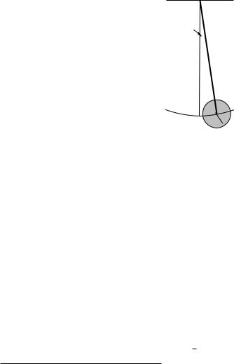
Figure 119: A simple pendulum is just a point like mass suspended on a long string and displaced sideways by a small angle. We will assume no damping forces and that there is no initial velocity into or out of the page, so that the motion is stricly in the plane of the page.

This is almost a simple harmonic equation. To make it one, we have to use the small angle approximation:

Now you see the advantage of all of our hard work in the last section. To solve any SHO problem one simply puts the di erential equation of motion (approximating as necessary) into the form of the SHO ODE which we have solved once and for all above! We can then just write down the solution and be quite confident that all of its features will be “just like” the features of the solution for a mass on a spring.

For example, if you compute the gravitational potential energy for the pendulum for arbitrary angle θ, you get:

This doesn’t initially look like the form we might expect from blindly substituting similar terms into the potential energy for mass on the spring, U (t) = 12 kx(t)2. “k” for the gravity problem is mω2, “x(t)” is θ(t), so:

is what we expect.

As an interesting and fun exercise (that really isn’t too di cult) see if you can prove that these two forms are really the same, if you make the small angle approximation θ 1 in the first form! This shows you pretty much where the approximation will break down as Θ is gradually increased. For large enough θ, the period of a pendulum clock does depend on the amplitude of the swing. This (and the next section) explains grandfather clocks – clocks with very long penduli that can swing very slowly through very small angles – and why they were so accurate for their day.

The negative sign is there because the torque opposes the angular displacement from equilibrium and points into the page as drawn.

Next we set this equal to Iα, where I is the total moment of inertia for the system about the pivot of the pendulum and simplify:

where we finish o with the small angle approximation as usual for pendulums. We can now recognize that this ODE has the standard form of the SHO ODE:

I left the result in terms of I because it is simpler that way, but of course we have to evaluate I in order to evaluate ω2. Using the parallel axis theorem (and/or the moment of inertia of a rod about a pivot through one end) we get:

This is “the moment of inertia of the rod plus the moment of inertia of the disk rotating about a parallel axis a distance ℓ away from its center of mass”. From this we can read o the angular frequency:

Note that the energy of this sort of pendulum can be tricky, not because it is conceptually any di erent from before but because there are so many symbols in the answer. For example, its potential energy is easy enough – it depends on the elevation of the center of masses of the rod and the disk.

where hopefully it is obvious that h(t) = ℓ/2 (1 − cos(θ(t))) and H(t) = ℓ (1 − cos(θ(t))) = 2h(t). Note that the time dependence is entirely inherited from the fact that θ(t) is a function of time.

The kinetic energy is given by:

where Ω = dθ/dt as usual.