1.3.2 Kirchhoff’s Laws

In formulating continuous system equations, Verilog-AMS HDL uses two sets of relationships. The first are the constitutive relationships which describe the behavior of each component. Constitutive relationships can be kept inside the simulator as built-in primitives or they can be provided by Verilog-AMS HDL module definitions.

The second set of relationships, interconnection relationships, describe the structure of the network. Interconnection relationships, which contain information on how the components are connected to each other, are only a function of the system topology. They are independent of the nature of the components.

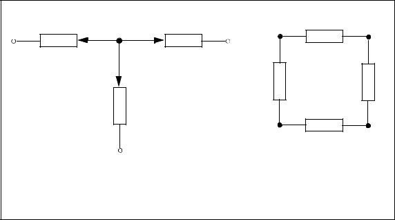
A Verilog-AMS HDL simulator uses Kirchhoff’s Laws to define the relationships between the nodes and the branches. Kirchhoff’s Laws are typically associated with electrical circuits that relate voltages and currents. However, by generalizing the concepts of voltages and currents to potentials and flows, Kirchhoff’s Laws can be used to formulate interconnection relationships for any type of system.

Kirchhoff’s Laws provide the following properties relating the quantities present on nodes and branches, as shown in Figure 1-3.

—Kirchhoff's Flow Law (KFL)

The algebraic sum of all flows out of a node at any instant is zero (0).

—Kirchhoff's Potential Law (KPL)

The algebraic sum of all the branch potentials around a loop at any instant is zero (0).

These laws imply a node is infinitely small; so there is negligible difference in potential between any two points on the node and a negligible accumulation of flow.

Figure 1-3: Kirchhoff’s Flow Law (KFL) and Potential Law (KPL)

1.3.3 Natures, disciplines, and nets

Verilog-AMS HDL allows definition of nets based on disciplines. The disciplines associate potential and flow natures for conservative systems or only potential nature for signal-flow systems. The natures are a collection of attributes, including user-defined attributes, which describes the units (meter, gram, newton, etc.), absolute tolerance for convergence, and the names of potential and flow access functions.

The disciplines and natures can be shared by many nets. The compatibility rules help enforce the legal operations between nets of different disciplines.

1.3.4 Signal-flow systems

A discipline may specify two nature bindings, potential and flow, or it may specify only a single binding, potential. Disciplines with two natures are know as conservative disciplines because nodes which are bound to them exhibit Kirchhoff’s Flow Law, and thus, conserve charge (in the electrical case). A discipline with only a potential nature is known as a signal flow discipline.

As a result of port connections of analog nets, a single node may be bound to a number of nets of different disciplines. If a node is bound only to disciplines which have potential nature only, current contributions to that node are not legal. Flow for such a node is not defined.

Signal flow models may be written so potentials of module outputs are purely functions of potentials at the inputs without taking flow into account.

The following example is a level shifting voltage follower:

module shiftPlus5(in, out); input in;

output out;

voltage in, out; //voltage is a signal flow //discipline compatible with //electrical, but having a //potential nature only

analog begin

V(out) <+ 5.0 + V(in); end

endmodule

If a number of such modules were cascaded in series, it would not be necessary to conserve charge (i.e., sum the flows) at any intervening node.

If, on the other hand, the output of this device were bound to a node of a conservative discipline (e.g., electrical), then the output of the device would appear to be a controlled voltage source to ground at that node. In that case, the flow (i.e., current) through the source would contribute to charge conservation at the node. If the input of this device were bound to a node of a conservative discipline then the input would act as a voltage probe to ground. Thus, when a net of signal flow discipline with potential nature only is bound to a conservative node, contributions made to that net behave as voltage sources to ground.

Nets of signal flow disciplines in modules may only be bound to input or output ports of the module, not to inout ports. Contributions may not be made to input ports.

1.3.5 Mixed conservative/signal flow systems

When practicing the top-down design style, it is extremely useful to mix conservative and signal-flow components in the same system. Users typically use signal-flow models early in the design cycle when the sys-

tem is described in abstract terms, and gradually convert component models to conservative form as the design progresses. Thus, it is important to be able to initially describe a component using a signal-flow model, and later convert it to a conservative model, with minimum changes. It is also important to allow conservative and signal-flow components to be arbitrarily mixed in the same system.

The approach taken is to write component descriptions using conservative semantics, except port and net declarations only require types for those values which are actually used in the description. Thus, signal-flow ports only require the type of potential to be specified, whereas conservative ports require types for both values (the potential and flow).

For example, consider a differential voltage amplifier, a differential current amplifier, and a resistor. The amplifiers are written using signal-flow ports and the resistor uses conservative ports.

module voltage_amplifier (out, in);

parameter real GAIN_V = 10.0;

analog

V(out) <+ GAIN_V * V(in);

endmodule

In this case, only the voltage on the ports are declared because only voltage is used in the body of the model.

module current_amplifier (out, in); input in;

parameter real GAIN_I = 10.0;

analog

I(out) <+ GAIN_I * I(in);

endmodule

Here, only current is used in the body of the model, so only current need be declared at the ports.

analog

V(a,b) <+ R * I(a,b);

endmodule

The description of the resistor relates both the voltage and current on the ports. Both are defined in the conservative discipline electrical.