0 V

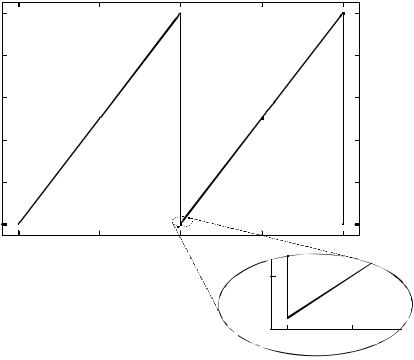
Figure 4-3: The output from the ramp generator

4.5.5 Circular integrator operator

The idtmod operator, also called the circular integrator, converts an expression argument into its indefinitely integrated form similar to the idt operator, as shown in Table 4-19.

Table 4-19—Circular integrator

Table 4-19—Circular integrator (continued)

The initial condition is optional. If the initial condition is not specified, it defaults to zero (0). Regardless, the initial condition shall force the DC solution to the system.

If idtmod() is used in a system with feedback configuration which forces expr to zero (0), the initial condition can be omitted without any unexpected behavior during simulation. For example, an operational amplifier alone needs an initial condition, but the same amplifier with the right external feedback circuitry does not need a forced DC solution.

The output of the idtmod() function shall remain in the range

offset <= idtmod < offset+modulus

The modulus shall be an expression which evaluates to a positive value. If the modulus is not specified, then idtmod() shall behave like idt() and not limit the output of the integrator.

The default for offset shall be zero (0).

The following relationship between idt() and idtmod() shall hold at all times.

If

y = idt(expr, ic);

z = idtmod(expr, ic, modulus, offset);

then

y = n * modulus + z; // n is an integer

where

offset ≤ z < modulus + offset

In this example, the circular integrator is useful in cases where the integral can get very large, such as a VCO. In a VCO, only the output values in the range [0,2π] are of interest, e.g.,

phase = idtmod(fc + gain*V(in), 0, 1, 0); V(OUT) <+ sin(2*‘M_PI*phase);

Here, the circular integrator returns a value in the range [0,1].

4.5.6 Derivative operator

ddx() provides access to symbolically-computed partial derivatives of expressions in the analog block. The analog simulator computes symbolic derivatives of expressions used in contribution statements in order to use Newton-Raphson iteration to solve the system of equations. In many cases in compact modeling, the

values of these derivatives are useful quantities for design, such as the trans conductance of a transistor (gm) or the capacitance of a nonlinear charge-storage element such as a varactor. The syntax for this operator is shown in Syntax 4-2.

The general form for the ddx() operator is:

ddx ( expr , unknown_quantity )

where:

—expr is the expression for which the symbolic derivative needs to be calculated.

—unknown_quantity is the branch probe (voltage or current probe) with respect to which the derivative of the expression needs to be computed.

The operator returns the partial derivative of its first argument with respect to the unknown indicated by the second argument, holding all other unknowns fixed and evaluated at the current operating point. The second argument shall be the potential of a scalar net or port or the flow through a branch, because these are the unknown variables in the system of equations for the analog solver. For the modified nodal analysis used in most SPICE-like simulators, these unknowns are the node voltages and certain branch currents.

If the expression does not depend explicitly on the unknown, then ddx() returns zero (0). Care must be taken when using implicit equations or indirect assignments, for which the simulator may create internal unknowns; derivatives with respect to these internal unknowns cannot be accessed with ddx().

Unlike the ddt() operator, no tolerance is required because the partial derivative is computed symbolically and evaluated at the current operating point.

This first example uses ddx() to obtain the conductance of the diode. The variable gdio is declared as an output variable (see 3.2.1) so that its value is available for inspection by the designer.

module diode(a,c); inout a, c; electrical a, c;

parameter real IS = 1.0e-14; real idio;

(*desc="small-signal conductance"*) real gdio;

analog begin

idio = IS * (limexp(V(a,c)/$vt) - 1); gdio = ddx(idio, V(a));

I(a,c) <+ idio; end

endmodule

The next example adds a series resistance to the diode using an implicit equation. Note that gdio does not represent the total conductance because the flow access I(a,c) requires introduction of another unknown in the system of equations. The conductance of the diode is properly reported as geff, which includes the effects of RS and the nonlinear equation.

module diode(a,c); inout a, c; electrical a, c;

parameter real IS = 1.0e-14; parameter real RS = 0.0; real idio, gdio;

(*desc="effective conductance"*)

The final example implements a voltage-controlled dependent current source and is used to illustrate the computations of partial derivatives.

module vccs(pout,nout,pin,nin); inout pout, nout, pin, nin; electrical pout, nout, pin, nin; parameter real k = 1.0;

real vin, one, minusone, zero; analog begin

vin = V(pin,nin);

one = ddx(vin, V(pin)); minusone = ddx(vin, V(nin)); zero = ddx(vin, V(pout)); I(pout,nout) <+ k * vin;

end endmodule

The names of the variables indicate the values of the partial derivatives: +1, -1, or 0. A SPICE-like simulator would use these values (scaled by the parameter k) in the Newton-Raphson solution method.

4.5.7 Absolute delay operator

absdelay() implements the absolute transport delay for continuous waveforms (use the transition() operator to delay discrete-valued waveforms). The general form is

absdelay ( input , td [ , maxdelay ] )

input is delayed by the amount td. In all cases td shall be a positive number. If the optional maxdelay is specified, then td can vary. If td becomes greater than maxdelay, maxdelay will be used as a substitute for td. If maxdelay is not specified, the value of td when the absdelay() is first evaluated shall be used and any future changes to td shall be ignored.

In DC and operating point analyses, absdelay() returns the value of its input. In AC and other small-sig- nal analyses, the absdelay() operator phase-shifts the input expression to the output of the delay operator based on the following formula.

Output(ω) = Input(ω) e–jωtd

td is evaluated as a constant at a particular time for any small signal analysis. In time-domain analyses, absdelay() introduces a transport delay equal to the instantaneous value of td based on the following formula.

Output(t) = Input(max(t – td, 0))