Part I: Getting Started with Excel

After performing these steps, a new icon appears on your Quick Access toolbar.

To use a data entry form, follow these steps:

1.Arrange your data so that Excel can recognize it as a table by entering headings for the columns in the first row of your data entry range.

2.Select any cell in the table and click the Form button on your Quick Access toolbar.

Excel displays a dialog box customized to your data (refer to Figure 2-7).

3.Fill in the information.

Press Tab to move between the text boxes. If a cell contains a formula, the formula result appears as text (not as an edit box). In other words, you can’t modify formulas using the data entry form.

4.When you complete the data form, click the New button.

Excel enters the data into a row in the worksheet and clears the dialog box for the next row of data.

Entering the current date or time into a cell

If you need to date-stamp or time-stamp your worksheet, Excel provides two shortcut keys that do this task for you:

•Current date: Ctrl+; (semicolon)

•Current time: Ctrl+Shift+; (semicolon)

The date and time are from the system time in your computer. If the date or time is not correct in Excel, use the Windows Control Panel to make the adjustment.

Note

When you use either of these shortcuts to enter a date or time into your worksheet, Excel enters a static value into the worksheet. In other words, the date or time entered doesn’t change when the worksheet is recalculated. In most cases, this setup is probably what you want, but you should be aware of this limitation. If you want the date or time display to update, use one of these formulas:

=TODAY()

=NOW()

Applying Number Formatting

Number formatting refers to the process of changing the appearance of values contained in cells. Excel provides a wide variety of number formatting options. In the following sections, you see how to use many of Excel’s formatting options to quickly improve the appearance of your worksheets.

42

Chapter 2: Entering and Editing Worksheet Data

Tip

The formatting that you apply works with the selected cell or cells. Therefore, you need to select the cell (or range of cells) before applying the formatting. Also remember that changing the number format does not affect the underlying value. Number formatting affects only the appearance. n

Values that you enter into cells normally are unformatted. In other words, they simply consist of a string of numerals. Typically, you want to format the numbers so that they’re easier to read or are more consistent in terms of the number of decimal places shown.

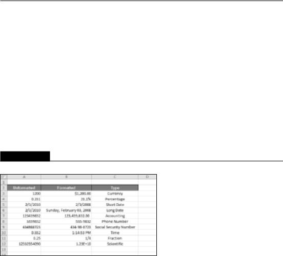
Figure 2.8 shows a worksheet that has two columns of values. The first column consists of unformatted values. The cells in the second column are formatted to make the values easier to read. The third column describes the type of formatting applied.

On the CD

This workbook is available on the companion CD-ROM. The file is named number formatting.xlsx.

FIGURE 2.8

Use numeric formatting to make it easier to understand what the values in the worksheet represent.

Tip

If you move the cell pointer to a cell that has a formatted value, the Formula bar displays the value in its unformatted state because the formatting affects only how the value appears in the cell — not the actual value contained in the cell. n

Using automatic number formatting

Excel is smart enough to perform some formatting for you automatically. For example, if you enter 12.2% into a cell, Excel knows that you want to use a percentage format and applies it for you automatically. If you use commas to separate thousands (such as 123,456), Excel applies comma formatting for you. And if you precede your value with a dollar sign, the cell is formatted for currency (assuming that the dollar sign is your system currency symbol).

43

Part I: Getting Started with Excel

Tip

A handy default feature in Excel makes entering percentage values into cells easier. If a cell is formatted to display as a percent, you can simply enter a normal value (for example, 12.5 for 12.5%). To enter values less than 1%, precede the value with a zero (for example, 0.52 for 0.52%). If this automatic percent–entry feature isn’t working (or if you prefer to enter the actual value for percents), access the Excel Options dialog box and click the Advanced tab. In the Editing Options section, locate the Enable Automatic Percent Entry check box and remove the check mark. n

Formatting numbers by using the Ribbon

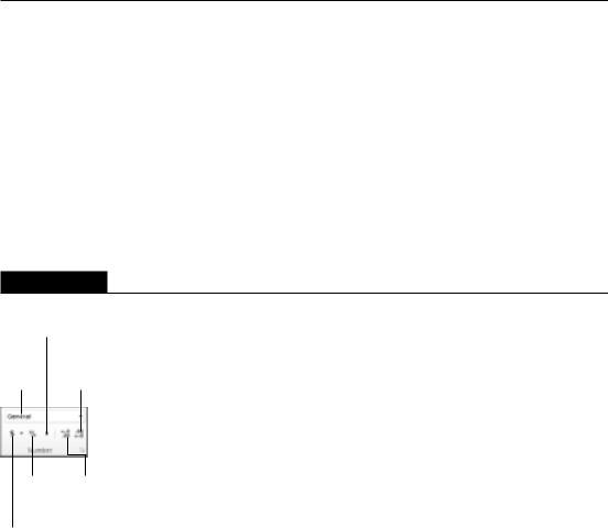
The Home Number group in the Ribbon contains controls that let you quickly apply common number formats (see Figure 2.9).

FIGURE 2.9

You can find number formatting commands in the Number group of the Home tab.

Comma Style

Decrease

Number Decimal

Format Places

Percent Increase

Style Decimal

Places

Accounting

Number

Format

The Number Format drop-down list contains 11 common number formats. Additional options include an Accounting Number Format drop-down list (to select a currency format), a Percent Style, and a Comma Style button. The group also contains a button to increase the number of decimal places, and another to decrease the number of decimal places.

When you select one of these controls, the active cell takes on the specified number format. You also can select a range of cells (or even an entire row or column) before clicking these buttons. If you select more than one cell, Excel applies the number format to all the selected cells.

44

Chapter 2: Entering and Editing Worksheet Data

Using shortcut keys to format numbers

Another way to apply number formatting is to use shortcut keys. Table 2.1 summarizes the short- cut-key combinations that you can use to apply common number formatting to the selected cells or range. Notice that these Ctrl+Shift characters are all located together, in the upper left of your keyboard.

TABLE 2.1

Formatting numbers using the Format Cells dialog box

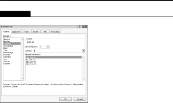
In most cases, the number formats that are accessible from the Number group on the Home tab are just fine. Sometimes, however, you want more control over how your values appear. Excel offers a great deal of control over number formats through the use of the Format Cells dialog box, shown in Figure 2.10. For formatting numbers, you need to use the Number tab.

You can bring up the Format Cells dialog box in several ways. Start by selecting the cell or cells that you want to format and then do one of the following:

•Choose Home Number and click the small dialog box launcher icon (in the lower-right corner of the Number group).

•Choose Home Number, click the Number Format drop-down list, and choose More Number Formats from the drop-down list.

•Right-click the cell and choose Format Cells from the shortcut menu.

•Press Ctrl+1.

45

Part I: Getting Started with Excel

FIGURE 2.10

When you need more control over number formats, use the Number tab of the Format Cells dialog box.

The Number tab of the Format Cells dialog box displays 12 categories of number formats from which to choose. When you select a category from the list box, the right side of the tab changes to display the appropriate options.

The Number category has three options that you can control: the number of decimal places displayed, whether to use a thousands separator, and how you want negative numbers displayed. Notice that the Negative Numbers list box has four choices (two of which display negative values in red), and the choices change depending on the number of decimal places and whether you choose to separate thousands.

The top of the tab displays a sample of how the active cell will appear with the selected number format (visible only if a cell with a value is selected). After you make your choices, click OK to apply the number format to all the selected cells.

Cross-Reference

Chapter 10 discusses ROUND and other built-in functions. n

The following are the number-format categories, along with some general comments:

•General: The default format; it displays numbers as integers, as decimals, or in scientific notation if the value is too wide to fit in the cell.

46

Chapter 2: Entering and Editing Worksheet Data

•Number: Enables you to specify the number of decimal places, whether to use a comma to separate thousands, and how to display negative numbers (with a minus sign, in red, in parentheses, or in red and in parentheses).

•Currency: Enables you to specify the number of decimal places, whether to use a currency symbol, and how to display negative numbers (with a minus sign, in red, in parentheses, or in red and in parentheses). This format always uses a comma to separate thousands.

•Accounting: Differs from the Currency format in that the currency symbols always align vertically.

•Date: Enables you to choose from several different date formats.

•Time: Enables you to choose from several different time formats.

•Percentage: Enables you to choose the number of decimal places and always displays a percent sign.

•Fraction: Enables you to choose from among nine fraction formats.

•Scientific: Displays numbers in exponential notation (with an E): 2.00E+05 = 200,000; 2.05E+05 = 205,000. You can choose the number of decimal places to display to the left of E.

•Text: When applied to a value, causes Excel to treat the value as text (even if it looks like a number). This feature is useful for such items as part numbers.

•Special: Contains additional number formats. In the U.S. version of Excel, the additional number formats are Zip Code, Zip Code +4, Phone Number, and Social Security Number.

•Custom: Enables you to define custom number formats that aren’t included in any other category.

Tip

If a cell displays a series of hash marks (such as #########), it usually means that the column isn’t wide enough to display the value in the number format that you selected. Either make the column wider or change the number format. n

Adding your own custom number formats

Sometimes you may want to display numerical values in a format that isn’t included in any of the other categories. If so, the answer is to create your own custom format.

Cross-Reference

Excel provides you with a great deal of flexibility in creating number formats — so much so that I’ve devoted an entire chapter (Chapter 24) to this topic. n

47

Part I: Getting Started with Excel

When Numbers Appear to Add Incorrectly

Applying a number format to a cell doesn’t change the value — only how the value appears in the worksheet. For example, if a cell contains 0.874543, you may format it to appear as 87%. If that cell is used in a formula, the formula uses the full value (0.874543), not the displayed value (87%).

In some situations, formatting may cause Excel to display calculation results that appear incorrect, such as when totaling numbers with decimal places. For example, if values are formatted to display two decimal places, you may not see the actual numbers used in the calculations. But because Excel uses the full precision of the values in its formula, the sum of the two values may appear to be incorrect.

Several solutions to this problem are available. You can format the cells to display more decimal places. You can use the ROUND function on individual numbers and specify the number of decimal places Excel should round to. Or you can instruct Excel to change the worksheet values to match their displayed format. To do so, access the Excel Options dialog box and click the Advanced tab. Check the Set Precision as Displayed check box (is located in the When Calculating This Workbook section).

Caution

Selecting the Precision as Displayed option changes the numbers in your worksheets to permanently match their appearance onscreen. This setting applies to all sheets in the active workbook. Most of the time, this option is not what you want. Make sure that you understand the consequences of using the Set Precision as Displayed option. n

48

CHAPTER

Essential Worksheet

Operations

49

Part I: Getting Started with Excel

Figure 3.1 shows Excel with four workbooks open, each in a separate window. One of the windows is minimized and appears near the lower-left corner of the screen. (When a workbook is minimized, only its title bar is visible.) Worksheet windows can overlap, and the title bar of one window is a different color. That’s the window that contains the active workbook.

FIGURE 3.1

You can open several Excel workbooks at the same time.

The workbook windows that Excel uses work much like the windows in any other Windows program. Each window has three buttons at the right side of its title bar. From left to right, they are Minimize, Maximize (or Restore), and Close. When a workbook window is maximized, the three buttons appear directly below the Excel title bar.

Workbook windows can be in one of the following states:

50

Chapter 3: Essential Worksheet Operations

•Maximized: Fills the entire Excel workspace. A maximized window doesn’t have a title bar, and the workbook’s name appears in the title bar for Excel. To maximize a window, click its Maximize button.

•Minimized: Appears as a small window with only a title bar. To minimize a window, click its Minimize button.

•Restored: A nonmaximized size. To restore a maximized or minimized window, click its Restore button.

If you work with more than one workbook simultaneously (which is quite common), you need to know how to move, resize, and switch among the workbook windows.

Moving and resizing windows

To move a window, make sure that it’s not maximized. Then click and drag its title bar with your mouse.

To resize a window, click and drag any of its borders until it’s the size that you want it to be. When you position the mouse pointer on a window’s border, the mouse pointer changes to a doublesided arrow, which lets you know that you can now click and drag to resize the window. To resize a window horizontally and vertically at the same time, click and drag any of its corners.

Note

You can’t move or resize a workbook window if it’s maximized. You can move a minimized window, but doing so has no effect on its position when it’s subsequently restored. n

If you want all your workbook windows to be visible (that is, not obscured by another window), you can move and resize the windows manually, or you can let Excel do it for you. Choosing View Window Arrange All displays the Arrange Windows dialog box, shown in Figure 3.2. This dialog box has four window-arrangement options. Just select the one that you want and click OK. Windows that are minimized aren’t affected by this command.

FIGURE 3.2

Use the Arrange Windows dialog box to quickly arrange all open non-minimized workbook windows.

51

Part I: Getting Started with Excel

Switching among windows

At any given time, one (and only one) workbook window is the active window. The active window accepts your input and is the window on which your commands work. The active window’s title bar is a different color, and the window appears at the top of the stack of windows. To work in a different window, you need to make that window active. You can make a different window the active workbook in several ways:

•Click another window, if it’s visible. The window you click moves to the top and becomes the active window. This method isn’t possible if the current window is maximized.

•Press Ctrl+Tab (or Ctrl+F6) to cycle through all open windows until the window that you want to work with appears on top as the active window. Pressing Shift+Ctrl+Tab (or Shift+Ctrl+F6) cycles through the windows in the opposite direction.

•Choose View Window Switch Windows and select the window that you want from the drop-down list (the active window has a check mark next to it). This menu can display as many as nine windows. If you have more than nine workbook windows open, choose More Windows (which appears below the nine window names).

•Click the icon for the window in the Windows taskbar. This technique is available only if the Show All Windows in the Taskbar option is turned on. You can control this setting from the Advanced tab of the Excel Options dialog box (in the Display section).

Tip

Most people prefer to do most of their work with maximized workbook windows, which enables you to see more cells and eliminates the distraction of other workbook windows getting in the way. At times, however, viewing multiple windows is preferred. For example, displaying two windows is more efficient if you need to compare information in two workbooks or if you need to copy data from one workbook to another. n

When you maximize one window, all the other windows are maximized, too (even though you don’t see them). Therefore, if the active window is maximized and you activate a different window, the new active window is also maximized.

Tip

You also can display a single workbook in more than one window. For example, if you have a workbook with two worksheets, you may want to display each worksheet in a separate window to compare the two sheets. All the window-manipulation procedures described previously still apply. Choose View Window New Window to open an additional window in the active workbook. n

Closing windows

If you have multiple windows open, you may want to close those windows that you no longer need. Excel offers several ways to close the active window:

52

Chapter 3: Essential Worksheet Operations

•Choose File Close.

•Click the Close button (the X icon) on the workbook window’s title bar. If the workbook window is maximized, its title bar is not visible, so its Close button appears directly below the Excel Close button.

•Press Ctrl+W.

When you close a workbook window, Excel checks whether you made any changes since the last time you saved the file. If you have made changes, Excel prompts you to save the file before it closes the window. If not, the window closes without a prompt from Excel.

Activating a worksheet

At any given time, one workbook is the active workbook, and one sheet is the active sheet in the active workbook. To activate a different sheet, just click its sheet tab, located at the bottom of the workbook window. You also can use the following shortcut keys to activate a different sheet:

•Ctrl+PgUp: Activates the previous sheet, if one exists

•Ctrl+PgDn: Activates the next sheet, if one exists

If your workbook has many sheets, all its tabs may not be visible. Use the tab scrolling controls (see Figure 3.3) to scroll the sheet tabs. The sheet tabs share space with the worksheet’s horizontal scroll bar. You also can drag the tab split control to display more or fewer tabs. Dragging the tab split control simultaneously changes the number of tabs and the size of the horizontal scroll bar.

Tip

When you right-click any of the tab scrolling controls, Excel displays a list of all sheets in the workbook. You can quickly activate a sheet by selecting it from the list. n

FIGURE 3.3

Use the tab controls to activate a different worksheet or to see additional worksheet tabs.

53

Part I: Getting Started with Excel

Adding a new worksheet to your workbook

Worksheets can be an excellent organizational tool. Instead of placing everything on a single worksheet, you can use additional worksheets in a workbook to separate various workbook elements logically. For example, if you have several products whose sales you track individually, you may want to assign each product to its own worksheet and then use another worksheet to consolidate your results.

The following are three ways to add a new worksheet to a workbook:

•Click the Insert Worksheet control, which is located to the right of the last sheet tab. This method inserts the new sheet after the last sheet in the workbook.

•Press Shift+F11. This method inserts the new sheet before the active sheet.

•Right-click a sheet tab, choose Insert from the shortcut menu, and click the General tab of the Insert dialog box that appears. Then select the Worksheet icon and click OK. This method inserts the new sheet before the active sheet.

Deleting a worksheet you no longer need

If you no longer need a worksheet, or if you want to get rid of an empty worksheet in a workbook, you can delete it in either of two ways:

•Right-click its sheet tab and choose Delete from the shortcut menu.

•Activate the unwanted worksheet and choose Home Cells Delete Delete Sheet. If the worksheet contains any data, Excel asks you to confirm that you want to delete the sheet. If you’ve never used the worksheet, Excel deletes it immediately without asking for confirmation.

Tip

You can delete multiple sheets with a single command by selecting the sheets that you want to delete. To select multiple sheets, press Ctrl while you click the sheet tabs that you want to delete. To select a group of contiguous sheets, click the first sheet tab, press Shift, and then click the last sheet tab. Then use either method to delete the selected sheets. n

Caution

When you delete a worksheet, it’s gone for good. Deleting a worksheet is one of the few operations in Excel that can’t be undone. n

Changing the name of a worksheet

The default names that Excel uses for worksheets — Sheet1, Sheet2, and so on — aren’t very descriptive. If you don’t change the worksheet names, remembering where to find things in multi- ple-sheet workbooks can be a bit difficult. That’s why providing more meaningful names for your worksheets is often a good idea.

54

Chapter 3: Essential Worksheet Operations

Changing the Default Number of Sheets

in Your Workbooks

By default, Excel automatically creates three worksheets in each new workbook. You can change this default behavior. For example, I prefer to start each new workbook with a single worksheet. After all, you can easily add new sheets if and when they’re needed. To change the default number of worksheets:

1.Choose File Excel Options to display the Excel Options window.

2.Click the General tab.

3.Change the value for the Include This Many Sheets setting and then click OK.

Making this change affects all new workbooks but has no effect on existing workbooks.

To change a sheet’s name, double-click the sheet tab. Excel highlights the name on the sheet tab so that you can edit the name or replace it with a new name.

Sheet names can be up to 31 characters, and spaces are allowed. However, you can’t use the following characters in sheet names:

:colon

/ slash

\ backslash

[ ] square brackets

< > angle brackets

.period

? question mark

’ apostrophe

* asterisk

Keep in mind that a longer worksheet name results in a wider tab, which takes up more space onscreen. Therefore, if you use lengthy sheet names, you won’t be able to see very many sheet tabs without scrolling the tab list.

Changing a sheet tab color

Excel allows you to change the color of your worksheet tabs. For example, you may prefer to color-code the sheet tabs to make identifying the worksheet’s contents easier.

55

Part I: Getting Started with Excel

To change the color of a sheet tab, right-click the tab and choose Tab Color from the shortcut menu. Then select the color from the color selector box.

Rearranging your worksheets

You may want to rearrange the order of worksheets in a workbook. If you have a separate worksheet for each sales region, for example, arranging the worksheets in alphabetical order may be helpful. You may want to move a worksheet from one workbook to another. (To move a worksheet to a different workbook, both workbooks must be open.) You can also create copies of worksheets.

You can move or copy a worksheet in the following ways:

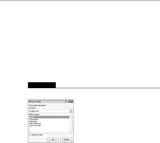
•Right-click the sheet tab and choose Move or Copy to display the Move or Copy dialog box (see Figure 3.4). Use this dialog box to specify the operation and the location for the sheet.

FIGURE 3.4

Use the Move or Copy dialog box to move or copy worksheets in the same or another workbook.

•To move a worksheet, click the worksheet tab and drag it to its desired location (either in the same workbook or in a different workbook). When you drag, the mouse pointer changes to a small sheet, and a small arrow guides you.

•To copy a worksheet, click the worksheet tab, and press Ctrl while dragging the tab to its desired location (either in the same workbook or in a different workbook). When you drag, the mouse pointer changes to a small sheet with a plus sign on it.

Tip

You can move or copy multiple sheets simultaneously. First select the sheets by clicking their sheet tabs while holding down the Ctrl key. Then you can move or copy the set of sheets by using the preceding methods. n

56

Chapter 3: Essential Worksheet Operations

If you move or copy a worksheet to a workbook that already has a sheet with the same name, Excel changes the name to make it unique. For example, Sheet1 becomes Sheet1 (2). You probably want to rename the copied sheet to give it a more meaningful. See “Changing the name of a worksheet,” earlier in this chapter.

Note

When you move or copy a worksheet to a different workbook, any defined names and custom formats also get copied to the new workbook. n

Hiding and unhiding a worksheet

In some situations, you may want to hide one or more worksheets. Hiding a sheet may be useful if you don’t want others to see it or if you just want to get it out of the way. When a sheet is hidden, its sheet tab is also hidden. You can’t hide all the sheets in a workbook; at least one sheet must remain visible.

To hide a worksheet, right-click its sheet tab and choose Hide Sheet. The active worksheet (or selected worksheets) will be hidden from view.

Preventing Sheet Actions

To prevent others from unhiding hidden sheets, inserting new sheets, renaming sheets, copying sheets, or deleting sheets, protect the workbook’s structure:

1.Choose Review Changes Protect Workbook.

2.In the Protect Workbook dialog box, click the Structure option.

3.(Optional) Provide a password.

After performing these steps, several commands will no longer be available when you right-click a sheet tab: Insert, Delete Sheet, Rename Sheet, Move or Copy Sheet, Tab Color, Hide Sheet, and Unhide Sheet. Be aware, however, that this is a very weak security measure. Cracking Excel’s protection features is relatively easy.

You can also make a sheet “very hidden.” A sheet that is very hidden doesn’t appear in the Unhide dialog box. To make a sheet very hidden:

1.Activate the worksheet.

2.Choose Developer Controls Properties. The Properties dialog box, shown in the following figure, appears. (If the Developer tab isn’t available, you can turn it on using the Customize Ribbon tab of the Excel Options dialog box.)

3.In the Properties box, select the Visible option and choose 2 - xlSheetVeryHidden.

continued

57