CHAPTER

Working with Cells and Ranges

69

Part I: Getting Started with Excel

Selecting ranges

To perform an operation on a range of cells in a worksheet, you must first select the range. For example, if you want to make the text bold for a range of cells, you must select the range and then choose Home Font Bold (or press Ctrl+B).

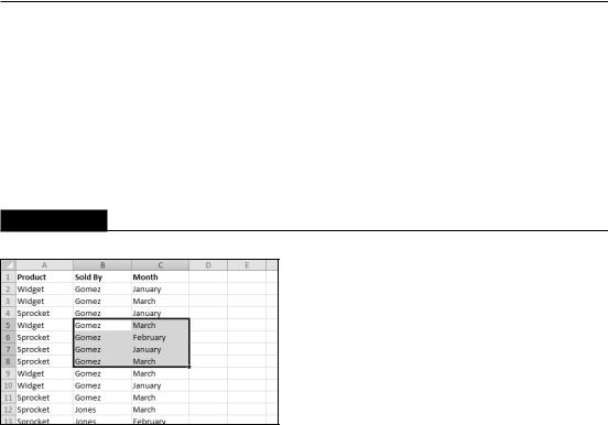
When you select a range, the cells appear highlighted. The exception is the active cell, which remains its normal color. Figure 4.1 shows an example of a selected range (B5:C8) in a worksheet. Cell B5, the active cell, is selected but not highlighted.

FIGURE 4.1

When you select a range, it appears highlighted, but the active cell within the range is not highlighted.

You can select a range in several ways:

•Press the left mouse button and drag, highlighting the range. Then release the mouse button. If you drag to the end of the screen, the worksheet will scroll.

•Press the Shift key while you use the navigation keys to select a range.

•Press F8 and then move the cell pointer with the navigation keys to highlight the range. Press F8 again to return the navigation keys to normal movement.

•Type the cell or range address into the Name box and press Enter. Excel selects the cell or range that you specified.

•Choose Home Editing Find & Select Go To (or press F5) and enter a range’s address manually into the Go To dialog box. When you click OK, Excel selects the cells in the range that you specified.

Tip

While you’re selecting a range, Excel displays the number of rows and columns in your selection in the Name box (located on the left side of the Formula bar). As soon as you finish the selection, the Name box reverts to showing the address of the active cell. n

70

Chapter 4: Working with Cells and Ranges

Selecting complete rows and columns

Often, you’ll need to select an entire row or column. For example, you may want to apply the same numeric format or the same alignment options to an entire row or column. You can select entire rows and columns in much the same manner as you select ranges:

•Click the row or column border to select a single row or column.

•To select multiple adjacent rows or columns, click a row or column border and drag to highlight additional rows or columns.

•To select multiple (nonadjacent) rows or columns, press Ctrl while you click the row or column borders that you want.

•Press Ctrl+spacebar to select a column. The column of the active cell (or columns of the selected cells) is highlighted.

•Press Shift+spacebar to select a row. The row of the active cell (or rows of the selected cells) is highlighted.

Tip

Press Ctrl+A to select all cells in the worksheet, which is the same as selecting all rows and all columns. If the active cell is within a table, you may need to press Ctrl+A two or even three times to select all cells in the worksheet. You can also click the area at the intersection of the row and column borders to select all cells. n

Selecting noncontiguous ranges

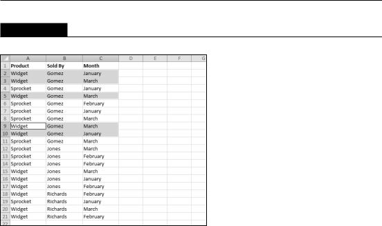
Most of the time, the ranges that you select are contiguous — a single rectangle of cells. Excel also enables you to work with noncontiguous ranges, which consist of two or more ranges (or single cells) that aren’t next to each other. Selecting noncontiguous ranges is also known as a multiple selection. If you want to apply the same formatting to cells in different areas of your worksheet, one approach is to make a multiple selection. When the appropriate cells or ranges are selected, the formatting that you select is applied to them all. Figure 4.2 shows a noncontiguous range selected in a worksheet. Three ranges are selected: A2:C3, A5:C5, and A9:C10.

You can select a noncontiguous range in several ways:

•Select the first range (or cell). Then press and hold Ctrl as you click and drag the mouse to highlight additional cells or ranges.

•From the keyboard, select a range as described previously (using F8 or the Shift key). Then press Shift+F8 to select another range without canceling the previous range selections.

•Enter the range (or cell) address in the Name box and press Enter. Separate each range address with a comma.

•Choose Home Editing Find & Select Go To (or press F5) to display the Go To dialog box. Enter the range (or cell) address in the Reference box and separate each range address with a comma. Click OK, and Excel selects the ranges.

71

Part I: Getting Started with Excel

FIGURE 4.2

Excel enables you to select noncontiguous ranges.

Note

Noncontiguous ranges differ from contiguous ranges in several important ways. One obvious difference is that you can’t use drag-and-drop methods (described later) to move or copy noncontiguous ranges. n

Selecting multisheet ranges

In addition to two-dimensional ranges on a single worksheet, ranges can extend across multiple worksheets to be three-dimensional ranges.

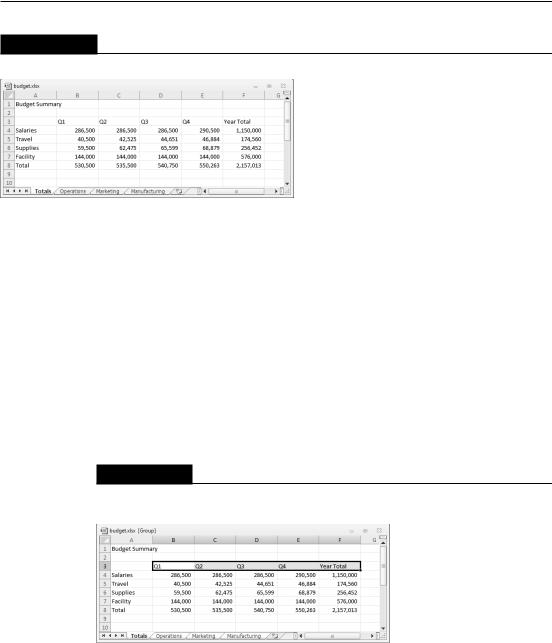
Suppose that you have a workbook set up to track budgets. A common approach is to use a separate worksheet for each department, making it easy to organize the data. You can click a sheet tab to view the information for a particular department.

Figure 4.3 shows a simplified example. The workbook has four sheets: Totals, Operations, Marketing, and Manufacturing. The sheets are laid out identically. The only difference is the values. The Totals sheet contains formulas that compute the sum of the corresponding items in the three departmental worksheets.

On the CD

This workbook, named budget.xlsx, is available on the companion CD-ROM. n

72

Chapter 4: Working with Cells and Ranges

FIGURE 4.3

The worksheets in this workbook are laid out identically.

Assume that you want to apply formatting to the sheets — for example, make the column headings bold with background shading. One (albeit not-so-efficient) approach is to format the cells in each worksheet separately. A better technique is to select a multisheet range and format the cells in all the sheets simultaneously. The following is a step-by-step example of multisheet formatting, using the workbook shown in Figure 4.3.

1.Activate the Totals worksheet by clicking its tab.

2.Select the range B3:F3.

3.Press Shift and click the Manufacturing sheet tab. This step selects all worksheets between the active worksheet (Totals) and the sheet tab that you click — in essence, a three-dimensional range of cells (see Figure 4.4). Notice that the workbook window’s title bar displays [Group] to remind you that you’ve selected a group of sheets and that you’re in Group mode.

FIGURE 4.4

In Group mode, you can work with a three-dimensional range of cells that extend across multiple worksheets.

73

Part I: Getting Started with Excel

4.Choose Home Font Bold and then choose Home Font Fill Color to apply a colored background. Excel applies the formatting to the selected range across the selected sheets.

5.Click one of the other sheet tabs. This step selects the sheet and also cancels Group mode; [Group] is no longer displayed in the title bar.

When a workbook is in Group mode, any changes that you make to cells in one worksheet also apply to all the other grouped worksheets. You can use this to your advantage when you want to set up a group of identical worksheets because any labels, data, formatting, or formulas you enter are automatically added to the same cells in all the grouped worksheets.

Note

When Excel is in Group mode, some commands are disabled and can’t be used. In the preceding example, you can’t convert all these ranges to tables by choosing Insert Tables Table. n

In general, selecting a multisheet range is a simple two-step process: Select the range in one sheet and then select the worksheets to include in the range. To select a group of contiguous worksheets, you can press Shift and click the sheet tab of the last worksheet that you want to include in the selection. To select individual worksheets, press Ctrl and click the sheet tab of each worksheet that you want to select. If all the worksheets in a workbook aren’t laid out the same, you can skip the sheets that you don’t want to format. When you make the selection, the sheet tabs of the selected sheets appear with a white background, and Excel displays [Group] in the title bar.

Tip

To select all sheets in a workbook, right-click any sheet tab and choose Select All Sheets from the shortcut menu. n

Selecting special types of cells

As you use Excel, you may need to locate specific types of cells in your worksheets. For example, wouldn’t it be handy to be able to locate every cell that contains a formula — or perhaps all the cells whose value depends on the current cell? Excel provides an easy way to locate these and many other special types of cells. Simply choose Home Editing Find & Select Go to Special to display the Go to Special dialog box, shown in Figure 4.5.

After you make your choice in the dialog box, Excel selects the qualifying subset of cells in the current selection. Often, this subset of cells is a multiple selection. If no cells qualify, Excel lets you know with the message No cells were found.

Tip

If you bring up the Go to Special dialog box with only one cell selected, Excel bases its selection on the entire used area of the worksheet. Otherwise, the selection is based on the selected range. n

74

Chapter 4: Working with Cells and Ranges

FIGURE 4.5

Use the Go to Special dialog box to select specific types of cells.

Table 4.1 offers a description of the options available in the Go to Special dialog box. Some of the options are very useful.

TABLE 4.1

75

Part I: Getting Started with Excel

Tip

When you select an option in the Go to Special dialog box, be sure to note which suboptions become available. For example, when you select Constants, the suboptions under Formulas become available to help you further refine the results. Likewise, the suboptions under Dependents also apply to Precedents, and those under Data Validation also apply to Conditional Formats. n

Selecting cells by searching

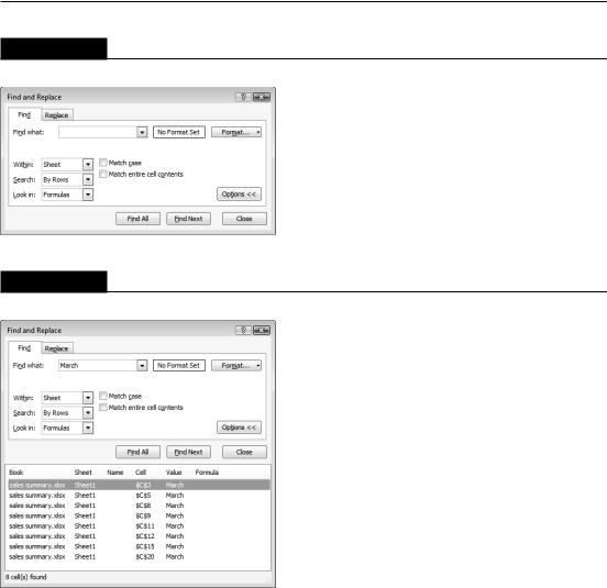
Another way to select cells is to use the Excel Home Editing Find & Select Find, command (or press Ctrl+F), which allows you to select cells by their contents. The Find and Replace dialog box is shown in Figure 4.6. This figure shows additional options that are available when you click the Options button.

Enter the text that you’re looking for; then click Find All. The dialog box expands to display all the cells that match your search criteria. For example, Figure 4.7 shows the dialog box after Excel has located all cells that contain the text March. You can click an item in the list, and the screen will scroll so that you can view the cell in context. To select all the cells in the list, first select any single item in the list. Then press Ctrl+A to select them all.

76

Chapter 4: Working with Cells and Ranges

FIGURE 4.6

The Find and Replace dialog box, with its options displayed.

FIGURE 4.7

The Find and Replace dialog box, with its results listed.

Note

The Find and Replace dialog box allows you to return to the worksheet without dismissing the dialog box. n

The Find and Replace dialog box supports two wildcard characters:

•? matches any single character.

•* matches any number of characters.

77