Chapter 37: Analyzing Data Using Goal Seeking and Solver

This list describes Solver’s options:

•Constraint Precision: Specify how close the Cell Reference and Constraint formulas must be to satisfy a constraint. Excel may solve the problem more quickly if you specify less precision.

•Use Automatic Scaling: Use when the problem involves large differences in magnitude — when you attempt to maximize a percentage, for example, by varying cells that are very large.

•Show Iteration Results: Instruct Solver to pause and display the results after each iteration by selecting this check box.

•Ignore Integer Constraints: When this check box is selected, Solver ignores constraints that specify that a particular cell must be an integer. Using this option may allow Solver to find a solution that cannot be found otherwise.

•Max Time: Specify the maximum amount of time (in seconds) that you want Solver to spend on a problem. If Solver reports that it exceeded the time limit, you can increase the amount of time that it spends searching for a solution.

•Iterations: Enter the maximum number of trial solutions that you want Solver to perform.

•Max Subproblems: For complex problems. Specify the maximum number of subproblems that may be explored by the Evolutionary algorithm.

•Max Feasible Solutions: For complex problems. Specify the maximum number of feasible solutions that may be explored by the Evolutionary algorithm.

Note

The other two tabs in the Options dialog box contain additional options used by the GRG Nonlinear and Evolutionary algorithms. n

Solver Examples

The remainder of this chapter consists of examples of using Solver for various types of problems.

Solving simultaneous linear equations

This example describes how to solve a set of three linear equations with three variables. Here’s an example of a set of linear equations:

4x + y -2z =0

2x - 3y +3z =9 -6x -2y +z = 0

The question that Solver will answer is What values of x, y, and z satisfy all three equations?

771

Part V: Analyzing Data with Excel

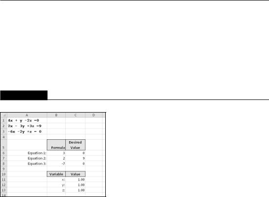
Figure 37.9 shows a workbook set up to solve this problem. This workbook has three named cells, which makes the formulas more readable:

•x: C11

•y: C12

•z: C13

The three named cells are all initialized to 1 (which certainly doesn’t solve the equations).

FIGURE 37.9

Solver will attempt to solve this series of linear equations.

On the CD

This workbook, named linear equations.xlsx, is available on the companion CD-ROM. n

The three equations are represented by formulas in the range B6:B8:

•B6: =(4*x)+(y)-(2*z)

•B7: =(2*x)-(3*y)+(3*z)

•B8: =-(6*x)-(2*y)+(z)

These formulas use the values in the x, y, and z named cells. The range C6:C8 contains the “desired” result for these three formulas.

Solver will adjust the values in x, y, and z — that is, the changing cells in C11:C13 — subject to these constraints:

•B6=C6

•B7=C7

•B8=C8

772

Chapter 37: Analyzing Data Using Goal Seeking and Solver

Note

This problem doesn’t have a target cell because it’s not trying to maximize or minimize anything. However, the Solver Parameters dialog box insists that you specify a formula for the Set Target Cell field. Therefore, just enter a reference to any cell that has a formula. n

Figure 37.10 shows the solution. The x (0.75), y (–2.0), and z (0.5) values satisfy all three equations.

FIGURE 37.10

Solver solved the simultaneous equations.

Note

A set of linear equations may have one solution, no solution, or an infinite number of solutions. n

Minimizing shipping costs

This example involves finding alternative options for shipping materials, while keeping total shipping costs at a minimum (see Figure 37.11). A company has warehouses in Los Angeles, St. Louis, and Boston. Retail outlets throughout the United States place orders, which the company then ships from one of the warehouses. The company wants to meet the product needs of all six retail outlets from available inventory and keep total shipping charges as low as possible.

On the CD

This workbook, named shipping costs.xlsx, is available on the companion CD-ROM. n

773

Part V: Analyzing Data with Excel

FIGURE 37.11

This worksheet determines the least expensive way to ship products from warehouses to retail outlets.

This workbook is rather complicated, so each part is explained individually:

•Shipping Costs Table: This table, in range B2:E8, is a matrix that contains per-unit shipping costs from each warehouse to each retail outlet. The cost to ship a unit from Los Angeles to Denver, for example, is $58.

•Product needs of each retail store: This information appears in C12:C17. For example, Denver needs 150 units, Houston needs 225, and so on. C18 contains a formula that calculates the total needed.

•Number to ship from: Range D12:F17 holds the adjustable cells that Solver varies. These cells are all initialized with a value of 25 to give Solver a starting value. Column G contains formulas that sum the number of units the company needs to ship to each retail outlet.

•Warehouse inventory: Row 21 contains the amount of inventory at each warehouse, and row 22 contains formulas that subtract the amount shipped (row 18) from the inventory.

•Calculated shipping costs: Row 24 contains formulas that calculate the shipping costs. Cell D24 contains the following formula, which is copied to the two cells to the right of Cell D24:

=SUMPRODUCT(C3:C8,D12:D17)

774

Chapter 37: Analyzing Data Using Goal Seeking and Solver

Cell G24 is the bottom line, the total shipping costs for all orders.

Solver fills in values in the range D12:F17 in such a way that minimizes shipping costs while still supplying each retail outlet with the desired number of units. In other words, the solution minimizes the value in cell G24 by adjusting the cells in D12:F17, subject to the following constraints:

•The number of units needed by each retail outlet must equal the number shipped. (In other words, all the orders are filled.) These constraints are represented by the following specifications:

C12=G12 C14=G14 C16=G16

C13=G13 C15=G15 C17=G17

•The adjustable cells can’t be negative because shipping a negative number of units makes no sense. These constraints are represented by the following specifications:

D12>=0 E12>=0 F12>=0

D13>=0 E13>=0 F13>=0

D14>=0 E14>=0 F14>=0

D15>=0 E15>=0 F15>=0

D16>=0 E16>=0 F16>=0

D17>=0 E17>=0 F17>=0

•The number of units remaining in each warehouse’s inventory must not be negative (that is, they can’t ship more than what’s available). This is represented by the following constraint specifications:

D22>=0 E22>=0 F22>=0

Note

Before you solve this problem with Solver, you may want to attempt to solve this problem manually, by entering values in D12:F17 that minimize the shipping costs. And, of course, you need to make sure that all the constraints are met. Doing so may help you better appreciate Solver. n

Setting up the problem is the difficult part. For example, you must enter 27 constraints. When you have specified all the necessary information, click the Solve button to put Solver to work. Solver displays the solution shown in Figure 37.12.

Learning More about Solver

Solver is a complex tool, and this chapter barely scratches the surface. If you’d like to learn more about Solver, I highly recommend the Web site for Frontline Systems:

www.solver.com

Frontline Systems is the company that developed Solver for Excel. Its Web site has several tutorials and lots of helpful information, including a detailed manual that you can download. You can also find additional Solver products for Excel that can handle much more complex problems.

775

Part V: Analyzing Data with Excel

The total shipping cost is $55,515, and all the constraints are met. Notice that shipments to Miami come from both St. Louis and Boston.

FIGURE 37.12

The solution that was created by Solver.

Allocating resources

The example in this section is a common type of problem that’s ideal for Solver. Essentially, problems of this sort involve optimizing the volumes of individual production units that use varying amounts of fixed resources. Figure 37.13 shows an example for a toy company.

On the CD

This workbook is available on the companion CD-ROM. The file is named allocating resources.xlsx.

This company makes five different toys, which use six different materials in varying amounts. For example, Toy A requires 3 units of blue paint, 2 units of white paint, 1 unit of plastic, 3 units of wood, and 1 unit of glue. Column G shows the current inventory of each type of material. Row 10 shows the unit profit for each toy.

776

Chapter 37: Analyzing Data Using Goal Seeking and Solver

FIGURE 37.13

Using Solver to maximize profit when resources are limited.

The number of toys to make is shown in the range B11:F11. These are the values that Solver determines (the changing cells). The goal of this example is to determine how to allocate the resources to maximize the total profit (B13). In other words, Solver determines how many units of each toy to make. The constraints in this example are relatively simple:

•Ensure that production doesn’t use more resources than are available. This can be accomplished by specifying that each cell in column I is greater than or equal to 0 (zero).

•Ensure that the quantities produced aren’t negative. This can be accomplished by specifying that each cell in row 11 be greater than or equal to 0.

Figure 37.14 shows the results that are produced by Solver. It shows the product mix that generates $12,365 in profit and uses all resources in their entirety, except for glue.

FIGURE 37.14

Solver determined how to use the resources to maximize the total profit.

777

Part V: Analyzing Data with Excel

Optimizing an investment portfolio

This example demonstrates how to use Solver to help maximize the return on an investment portfolio. A portfolio consists of several investments, each of which has a different yield. In addition, you may have some constraints that involve reducing risk and diversification goals. Without such constraints, a portfolio problem becomes a no-brainer: Put all your money in the investment with the highest yield.

This example involves a credit union (a financial institution that takes members’ deposits and invests them in loans to other members, bank CDs, and other types of investments). The credit union distributes part of the return on these investments to the members in the form of dividends, or interest on their deposits.

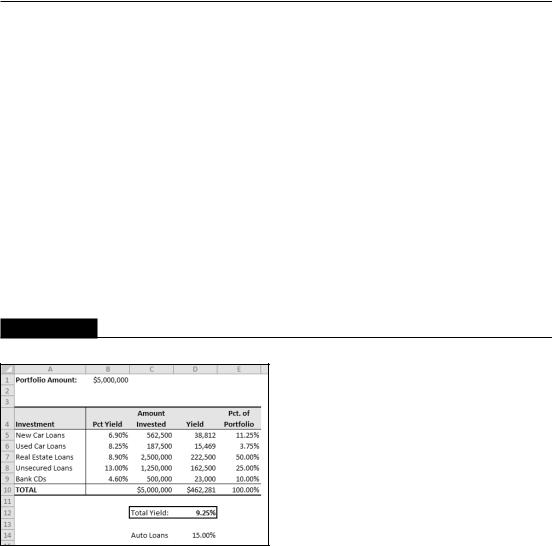
This hypothetical credit union must adhere to some regulations regarding its investments, and the board of directors has imposed some other restrictions. These regulations and restrictions comprise the problem’s constraints. Figure 37.15 shows a workbook set up for this problem.

FIGURE 37.15

This worksheet is set up to maximize a credit union’s investments, given some constraints.

On the CD

This workbook is available on the companion CD-ROM. The file is named investment portfolio.xlsx.

The following constraints are the ones to which you must adhere in allocating the $5 million portfolio:

•The amount that the credit union invests in new-car loans must be at least three times the amount that the credit union invests in used-car loans. (Used-car loans are riskier investments.) This constraint is represented as

C5>=C6*3

778

Chapter 37: Analyzing Data Using Goal Seeking and Solver

•Car loans should make up at least 15 percent of the portfolio. This constraint is represented as

D14>=.15

•Unsecured loans should make up no more than 25 percent of the portfolio. This constraint is represented as

E8<=.25

•At least 10 percent of the portfolio should be in bank CDs. This constraint is represented as:

E9>=.10

•The total amount invested is $5,000,000.

•All investments should be positive or zero. In other words, the problem requires five additional constraints to ensure that none of the changing cells goes below zero.

The changing cells are C5:C9, and the goal is to maximize the total yield in cell D12. Starting values of 1,000,000 have been entered in the changing cells. When you run Solver with these parameters, it produces the solution shown in Figure 37.16, which has a total yield of 9.25 percent.

FIGURE 37.16

The results of the portfolio optimization.

779

CHAPTER

Analyzing Data with the Analysis ToolPak

The Analysis ToolPak is an add-in that provides analytical capability that normally isn’t available.

Note

Prior to Excel 2007, the Analysis ToolPak add-in included many additional worksheet functions. These worksheet functions are built into Excel and no longer require the Analysis ToolPak add-in. n

These analysis tools offer many features that may be useful to those in the scientific, engineering, and educational communities — not to mention business users whose needs extend beyond the normal spreadsheet fare.

This section provides a quick overview of the types of analyses that you can perform with the Analysis ToolPak. This chapter covers each of the following tools:

•Analysis of variance (three types)

•Correlation

781