Chapter 18: Getting Started Making Charts

If you don’t want a particular embedded chart to appear on your printout, use the Properties tab of the Format Chart Area dialog box. To display this dialog box, double-click the background area of the chart. In the Properties tab of the Format Chart Area dialog box, clear the Print Object check box.

Understanding Chart Types

People who create charts usually do so to make a point or to communicate a specific message. Often, the message is explicitly stated in the chart’s title or in a text box within the chart. The chart itself provides visual support.

Choosing the correct chart type is often a key factor in the effectiveness of the message. Therefore, it’s often well worth your time to experiment with various chart types to determine which one conveys your message best.

In almost every case, the underlying message in a chart is some type of comparison. Examples of some general types of comparisons include

•Compare item to other items. A chart may compare sales in each of a company’s sales regions.

•Compare data over time. A chart may display sales by month and indicate trends over time.

•Make relative comparisons. A common pie chart can depict relative proportions in terms of pie “slices.”

•Compare data relationships. An XY chart is ideal for this comparison. For example, you might show the relationship between marketing expenditures and sales.

•Frequency comparison. You can use a common histogram, for example, to display the number (or percentage) of students who scored within a particular grade range.

•Identify “outliers” or unusual situations. If you have thousands of data points, creating a chart may help identify data that is not representative.

Choosing a chart type

A common question among Excel users is “How do I know which chart type to use for my data?” Unfortunately, this question has no cut-and-dried answer. Perhaps the best answer is a vague one: Use the chart type that gets your message across in the simplest way.

Figure 18.11 shows the same set of data plotted by using six different chart types. Although all six charts represent the same information (monthly Web site visitors), they look quite different from one another.

417

Part III: Creating Charts and Graphics

FIGURE 18.11

The same data, plotted by using six chart types.

On the CD

This workbook is available on the companion CD-ROM. The file is named six chart types.xlsx.

The column chart (upper left) is probably the best choice for this particular set of data because it clearly shows the information for each month in discrete units. The bar chart (upper right) is similar to a column chart, but the axes are swapped. Most people are more accustomed to seeing timebased information extend from left to right rather than from top to bottom.

The line chart (middle left) may not be the best choice because it seems to imply that the data is continuous — that points exist in between the 12 actual data points. This same argument may be made against using an area chart (middle right).

The pie chart (lower left) is simply too confusing and does nothing to convey the time-based nature of the data. Pie charts are most appropriate for a data series in which you want to emphasize proportions among a relatively small number of data points. If you have too many data points, a pie chart can be impossible to interpret.

418

Chapter 18: Getting Started Making Charts

The radar chart (lower right) is clearly inappropriate for this data. People aren’t accustomed to viewing time-based information in a circular direction!

Fortunately, changing a chart’s type is easy, so you can experiment with various chart types until you find the one that represents your data accurately, clearly, and as simply as possible.

The remainder of this chapter contains more information about the various Excel chart types. The examples and discussion may give you a better handle on determining the most appropriate chart type for your data.

Column

Probably the most common chart type is column charts. A column chart displays each data point as a vertical column, the height of which corresponds to the value. The value scale is displayed on the vertical axis, which is usually on the left side of the chart. You can specify any number of data series, and the corresponding data points from each series can be stacked on top of each other. Typically, each data series is depicted in a different color or pattern.

Column charts are often used to compare discrete items, and they can depict the differences between items in a series or items across multiple series. Excel offers seven column-chart subtypes.

On the CD

A workbook that contains the charts in this section is available on the companion CD-ROM. The file is named column charts.xlsx.

Figure 18.12 shows an example of a clustered column chart that depicts monthly sales for two products. From this chart, it is clear that Sprocket sales have always exceeded Widget sales. In addition, Widget sales have been declining over the five-month period, whereas Sprocket sales are increasing.

FIGURE 18.12

This clustered column chart compares monthly sales for two products.

419

Part III: Creating Charts and Graphics

The same data, in the form of a stacked column chart, is shown in Figure 18.13. This chart has the added advantage of depicting the combined sales over time. It shows that total sales have remained fairly steady each month, but the relative proportions of the two products have changed.

Figure 18.14 shows the same sales data plotted as a 100% stacked column chart. This chart type shows the relative contribution of each product by month. Notice that the vertical axis displays percentage values, not sales amounts. This chart provides no information about the actual sales volumes. This type of chart is often a good alternative to using several pie charts. Instead of using a pie to show the relative sales volume in each year, the chart uses a column for each year.

FIGURE 18.13

This stacked column chart displays sales by product and depicts the total sales.

FIGURE 18.14

This 100% stacked column chart display monthly sales as a percentage.

420

Chapter 18: Getting Started Making Charts

The data is plotted with a 3-D clustered column chart in Figure 18.15. The name is a bit deceptive, because the chart uses only two dimensions, not three. Many people use this type of chart because it has more visual pizzazz. Compare this chart with a “true” 3-D column chart, shown in Figure 18.16. This type of chart may be appealing visually, but precise comparisons are difficult because of the distorted perspective view.

You can also choose from column variations known as cylinder, cone, and pyramid charts. The only difference among these chart types and a standard column chart is the shape of the columns.

FIGURE 18.15

A 3-D column chart.

FIGURE 18.16

A true 3-D column chart.

421

Part III: Creating Charts and Graphics

Bar

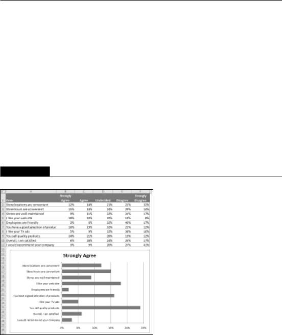
A bar chart is essentially a column chart that has been rotated 90 degrees clockwise. One distinct advantage to using a bar chart is that the category labels may be easier to read. Figure 18.17 shows a bar chart that displays a value for each of ten survey items. The category labels are lengthy, and displaying them legibly with a column chart would be difficult. Excel offers six bar chart subtypes.

On the CD

A workbook that contains the chart in this section is available on the companion CD-ROM. The file is named bar charts.xlsx.

Note

Unlike a column chart, no subtype displays multiple series along a third axis. (That is, Excel does not provide a 3-D Bar Chart subtype.) You can add a 3-D look to a column chart, but it will be limited to two axes. n

You can include any number of data series in a bar chart. In addition, the bars can be “stacked” from left to right.

FIGURE 18.17

If you have lengthy category labels, a bar chart may be a good choice.

422

Chapter 18: Getting Started Making Charts

Line

Line charts are often used to plot continuous data and are useful for identifying trends. For example, plotting daily sales as a line chart may enable you to identify sales fluctuations over time. Normally, the category axis for a line chart displays equal intervals. Excel supports seven line chart subtypes.

See Figure 18.18 for an example of a line chart that depicts daily sales (200 data points). Although the data varies quite a bit on a daily basis, the chart clearly depicts an upward trend.

On the CD

A workbook that contains the charts in this section is available on the companion CD-ROM. The file is named line charts.xlsx.

The final line chart example, shown in Figure 18.20, is a 3-D line chart. Although it has a nice visual appeal, it’s certainly not the clearest way to present the data. In fact, it’s fairly worthless.

A line chart can use any number of data series, and you distinguish the lines by using different colors, line styles, or markers. Figure 18.19 shows a line chart that has three series. The series are distinguished by markers (circles, squares, and diamonds) and different line colors.

FIGURE 18.18

A line chart often can help you spot trends in your data.

423

Part III: Creating Charts and Graphics

FIGURE 18.19

This line chart displays three series.

FIGURE 18.20

This 3-D line chart does not present the data very well.

Pie

A pie chart is useful when you want to show relative proportions or contributions to a whole. A pie chart uses only one data series. Pie charts are most effective with a small number of data points. Generally, a pie chart should use no more than five or six data points (or slices). A pie chart with too many data points can be very difficult to interpret.

424

Chapter 18: Getting Started Making Charts

Caution

The values used in a pie chart must all be positive numbers. If you create a pie chart that uses one or more negative values, the negative values will be converted to positive values — which is probably not what you intended! n

You can “explode” one or more slices of a pie chart for emphasis (see Figure 18.21). Activate the chart and click any pie slice to select the entire pie. Then click the slice that you want to explode and drag it away from the center.

On the CD

A workbook that contains the charts in this section is available on the companion CD-ROM. The file is named pie charts.xlsx.

FIGURE 18.21

A pie chart with one slice exploded.

The pie of pie and bar of pie chart types enables you to display a secondary chart that provides more detail for one of the pie slices. Figure 18.22 shows an example of a bar of pie chart. The pie chart shows the breakdown of four expense categories Rent, Supplies, Miscellaneous, and Salary. The secondary bar chart provides an additional regional breakdown of the Salary category.

The data used in the chart resides in A2:B8. When the chart was created, Excel made a guess at which categories belong to the secondary chart. In this case, the guess was to use the last three data points for the secondary chart — and the guess was incorrect.

To correct the chart, right-click any of the pie slices and choose Format Data Series. In the dialog box that appears, select the Series Options tab and make the changes. In this example, I chose Split Series by Position and specified that the Second Plot Contains the Last 4 Values in The Series.

425

Part III: Creating Charts and Graphics

FIGURE 18.22

A bar of pie chart that shows detail for one of the pie slices.

XY (scatter)

Another common chart type is an XY chart (also known as scattergrams or scatter plots). An XY chart differs from most other chart types in that both axes display values. (An XY chart has no category axis.)

This type of chart often is used to show the relationship between two variables. Figure 18.23 shows an example of an XY chart that plots the relationship between sales calls made (horizontal axis) and sales (vertical axis). Each point in the chart represents one month. The chart shows that these two variables are positively related: Months in which more calls were made typically had higher sales volumes.

FIGURE 18.23

An XY chart shows the relationship between two variables.

426

Chapter 18: Getting Started Making Charts

On the CD

A workbook that contains the charts in this section is available on the companion CD-ROM. The file is named xy charts.xlsx.

Note

Although these data points correspond to time, the chart doesn’t convey any time-related information. In other words, the data points are plotted based only on their two values. n

Figure 18.24 shows another XY chart, this one with lines that connect the XY points. This chart plots a hypocycloid curve with 200 data points. It’s set up with three parameters. Change any of the parameters, and you’ll get a completely different curve. This is a very minimalist chart. I deleted all the chart elements except the data series itself.

If this type of design looks familiar, it’s because a hypocycloid curve is the basis for a popular children’s drawing toy.

FIGURE 18.24

A hypocycloid curve, plotted as an XY chart.

Area

Think of an area chart as a line chart in which the area below the line has been colored in. Figure 18.25 shows an example of a stacked area chart. Stacking the data series enables you to see clearly the total, plus the contribution by each series.

427

Part III: Creating Charts and Graphics

FIGURE 18.25

A stacked area chart.

On the CD

A workbook that contains the charts in this section is available on the companion CD-ROM. The file is named area charts.xlsx.

Figure 18.26 shows the same data, plotted as a 3-D area chart. As you can see, it’s not an example of an effective chart. The data for products B and C are obscured. In some cases, the problem can be resolved by rotating the chart or using transparency. But usually the best way to salvage a chart like this is to select a new chart type.

FIGURE 18.26

This 3-D area chart is not a good choice.

428

Chapter 18: Getting Started Making Charts

Doughnut

A doughnut chart is similar to a pie chart, with two differences: It has a hole in the middle, and it can display more than one series of data. Doughnut charts are listed in the Other Charts category.

Figure 18.27 shows an example of a doughnut chart with two series (1st Half Sales and 2nd Half Sales). The legend identifies the data points. Because a doughnut chart doesn’t provide a direct way to identify the series, I added arrows and series descriptions manually.

On the CD

A workbook that contains the charts in this section is available on the companion CD-ROM. The file is named doughnut charts.xlsx.

FIGURE 18.27

A doughnut chart with two data series.

Notice that Excel displays the data series as concentric rings. As you can see, a doughnut chart with more than one series can be very difficult to interpret. For example, the relatively larger sizes of the slices toward the outer part of the doughnut can be deceiving. Consequently, you should use doughnut charts sparingly. Perhaps the best use for a doughnut chart is to plot a single series as a visual alternative to a pie chart.

In many cases, a stacked column chart for such comparisons expresses your meaning better than does a doughnut chart (see Figure 18.28).

429

Part III: Creating Charts and Graphics

FIGURE 18.28

Using a stacked column chart is a better choice.

Radar

Radar charts are listed in the Other Charts category. You may not be familiar with this type of chart. A radar chart is a specialized chart that has a separate axis for each category, and the axes extend outward from the center of the chart. The value of each data point is plotted on the corresponding axis.

Figure 18.29 shows an example of a radar chart. This chart plots two data series across 12 categories (months) and shows the seasonal demand for snow skis versus water skis. Note that the waterski series partially obscures the snow-ski series.

On the CD

A workbook that contains the charts in this section is available on the companion CD-ROM. The file is named radar charts.xlsx.

Using a radar chart to show seasonal sales may be an interesting approach, but it’s not the best. As you can see in Figure 18.30, a stacked bar chart shows the information much more clearly.

A more appropriate use for radar charts is shown in Figure 18.31. These four charts each plot a color. More precisely, each chart shows the RGB components (the contributions of red, green, and blue) that make up a color. Each chart has one series, and three categories. The categories extend from 0 to 255.

430

Chapter 18: Getting Started Making Charts

FIGURE 18.29

Plotting ski sales using a radar chart with 12 categories and 2 series.

FIGURE 18.30

A stacked bar chart is a better choice for the ski sales data.

Note

If you view the charts in color, you’ll see that they actually depict the color that they describe. The data series colors were applied manually. n

431

Part III: Creating Charts and Graphics

FIGURE 18.31

These radar charts depict the red, green, and blue contributions for each of four colors.

Surface

Surface charts display two or more data series on a surface. Surface charts are listed in the Other Charts category.

As Figure 18.32 shows, these charts can be quite interesting. Unlike other charts, Excel uses color to distinguish values, not to distinguish the data series. The number of colors used is determined by the major unit scale setting for the value axis. Each color corresponds to one major unit.

On the CD

A workbook that contains the charts in this section is available on the companion CD-ROM. The file is named surface charts.xlsx.

Note

A surface chart does not plot 3-D data points. The series axis for a surface chart, like with all other 3-D charts, is a category axis — not a value axis. In other words, if you have data that is represented by x, y, and z coordinates, it can’t be plotted accurately on a surface chart unless the x and y values are equally spaced. n

432

Chapter 18: Getting Started Making Charts

FIGURE 18.32

A surface chart.

Bubble

Think of a bubble chart as an XY chart that can display an additional data series, which is represented by the size of the bubbles. As with an XY chart, both axes are value axes (there is no category axis). Bubble charts are listed in the Other Charts category.

Figure 18.33 shows an example of a bubble chart that depicts the results of a weight-loss program. The horizontal value axis represents the original weight, the vertical value axis shows the number of weeks in the program, and the size of the bubbles represents the amount of weight lost.

On the CD

A workbook that contains the charts in this section is available on the companion CD-ROM. The file is named bubble charts.xlsx.

Figure 18.34 shows another bubble chart, made up of nine series that represent mouse face parts. The size and position of each bubble required some experimentation.

Stock

Stock charts are most useful for displaying stock-market information. These charts require three to five data series, depending on the subtype. This chart type is listed in the Other Charts category.

433

Part III: Creating Charts and Graphics

FIGURE 18.33

A bubble chart.

FIGURE 18.34

This bubble chart depicts a mouse.

Figure 18.35 shows an example of each of the four stock chart types. The two charts on the bottom display the trade volume and use two value axes. The daily volume, represented by columns, uses the axis on the left. The up-bars, sometimes referred to as candlesticks, are the vertical lines that

434

Chapter 18: Getting Started Making Charts

depict the difference between the opening and closing price. A black up-bar indicates that the closing price was lower than the opening price.

On the CD

A workbook that contains the charts in this section is available on the companion CD-ROM. The file is named stock charts.xlsx.

Stock charts aren’t just for stock price data. Figure 18.36 shows a chart that depicts the high, low, and average temperatures for each day in May. This is a high-low-close chart.

FIGURE 18.35

The four stock chart subtypes.

435