Chapter 4: Working with Cells and Ranges

Skipping blanks when pasting

The Skip Blanks option in the Paste Special dialog box prevents Excel from overwriting cell contents in your paste area with blank cells from the copied range. This option is useful if you’re copying a range to another area but don’t want the blank cells in the copied range to overwrite existing data.

Transposing a range

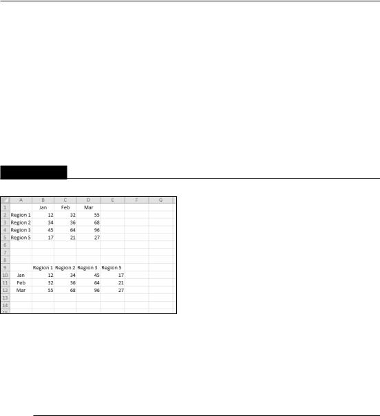
The Transpose option in the Paste Special dialog box changes the orientation of the copied range. Rows become columns, and columns become rows. Any formulas in the copied range are adjusted so that they work properly when transposed. Note that you can use this check box with the other options in the Paste Special dialog box. Figure 4.12 shows an example of a horizontal range (A1:D5) that was transposed to a different range (A9:E12).

FIGURE 4.12

Transposing a range changes the orientation as the information is pasted into the worksheet.

Tip

If you click the Paste Link button in the Paste Special dialog box, you create formulas that link to the source range. As a result, the destination range automatically reflects changes in the source range. n

Using Names to Work with Ranges

Dealing with cryptic cell and range addresses can sometimes be confusing. (This confusion becomes even more apparent when you deal with formulas, which I cover in Chapter 10.) Fortunately, Excel allows you to assign descriptive names to cells and ranges. For example, you can give a cell a name such as Interest_Rate, or you can name a range JulySales. Working with these names (rather than cell or range addresses) has several advantages:

89

Part I: Getting Started with Excel

•A meaningful range name (such as Total_Income) is much easier to remember than a cell address (such as AC21).

•Entering a name is less error-prone than entering a cell or range address.

•You can quickly move to areas of your worksheet either by using the Name box, located at the left side of the Formula bar (click the arrow to drop down a list of defined names) or by choosing Home Editing Find & Select Go To (or F5) and specifying the range name.

•Creating formulas is easier. You can paste a cell or range name into a formula by using Formula Autocomplete.

•Names make your formulas more understandable and easier to use. A formula such as

=Income—Taxes is more intuitive than =D20—D40.

Creating range names in your workbooks

Excel provides several different methods that you can use to create range names. Before you begin, however, you should be aware of some important rules about what is acceptable:

•Names can’t contain any spaces. You may want to use an underscore character to simulate a space (such as Annual_Total).

•You can use any combination of letters and numbers, but the name must begin with a letter. A name can’t begin with a number (such as 3rdQuarter) or look like a cell reference (such as QTR3). If these are desirable names, though, you can precede the name with an underscore: for example, _3rd Quarter and _QTR3.

•Symbols, except for underscores and periods, aren’t allowed.

•Names are limited to 255 characters, but it’s a good practice to keep names as short as possible yet still meaningful and understandable.

Caution

Excel also uses a few names internally for its own use. Although you can create names that override Excel’s internal names, you should avoid doing so. To be on the safe side, avoid using the following for names: Print_ Area, Print_Titles, Consolidate_Area, and Sheet_Title. To delete a range name or rename a range, see “Managing Names,” later in this chapter. n

Using the New Name dialog box

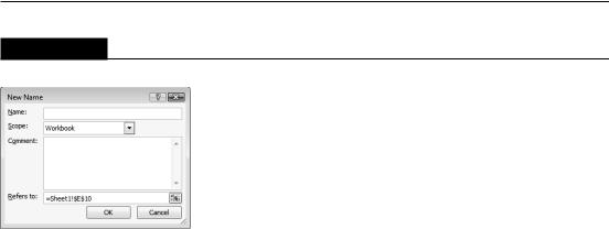
To create a range name, start by selecting the cell or range that you want to name. Then, choose Formulas Defined Names Define Name. Excel displays the New Name dialog box, shown in Figure 4.13. Note that this is a resizable dialog box. Click and drag a border to change the dimensions.

90

Chapter 4: Working with Cells and Ranges

FIGURE 4.13

Create names for cells or ranges by using the New Name dialog box.

Type a name in the Name text field (or use the name that Excel proposes, if any). The selected cell or range address appears in the Refers To text field. Use the Scope drop-down list to indicate the scope for the name. The scope indicates where the name will be valid, and it’s either the entire workbook or a particular sheet. If you like, you can add a comment that describes the named range or cell. Click OK to add the name to your workbook and close the dialog box.

Using the Name box

A faster way to create a name is to use the Name box (to the left of the Formula bar). Select the cell or range to name, click the Name box, and type the name. Press Enter to create the name. (You must press Enter to actually record the name; if you type a name and then click in the worksheet, Excel doesn’t create the name.) If a name already exists, you can’t use the Name box to change the range to which that name refers. Attempting to do so simply selects the range.

The Name box is a drop-down list and shows all names in the workbook. To choose a named cell or range, click the Name box and choose the name. The name appears in the Name box, and Excel selects the named cell or range in the worksheet.

Using the Create Names from Selection dialog box

You may have a worksheet that contains text that you want to use for names for adjacent cells or ranges. For example, you may want to use the text in column A to create names for the corresponding values in column B. Excel makes this task easy to do.

To create names by using adjacent text, start by selecting the name text and the cells that you want to name. (These items can be individual cells or ranges of cells.) The names must be adjacent to the cells that you’re naming. (A multiple selection is allowed.) Then, choose Formulas Defined Names Create from Selection. Excel displays the Create Names from Selection dialog box, shown in Figure 4.14. The check marks in this dialog box are based on Excel’s analysis of the selected range. For example, if Excel finds text in the first row of the selection, it proposes that you

91

Part I: Getting Started with Excel

create names based on the top row. If Excel didn’t guess correctly, you can change the check boxes. Click OK, and Excel creates the names. Using the data in Figure 4.14, Excel creates six names: January for cell B1, February for cell B2, and so on.

FIGURE 4.14

Use the Create Names from Selection dialog box to name cells using labels that appear in the worksheet.

Note

If the text contained in a cell would result in an invalid name, Excel modifies the name to make it valid. For example, if a cell contains the text Net Income (which is invalid for a name because it contains a space), Excel converts the space to an underscore character. If Excel encounters a value or a numeric formula where text should be, however, it doesn’t convert it to a valid name. It simply doesn’t create a name — and does not inform you of that fact. n

Caution

If the upper-left cell of the selection contains text and you choose the Top Row and Left Column options, Excel uses that text for the name of the entire data, excluding the top row and left column. So, after Excel creates the names, take a minute to make sure that they refer to the correct ranges. If Excel creates a name that is incorrect, you can delete or modify it by using the Name Manager (described next). n

Managing names

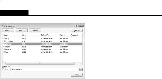
A workbook can have any number of names. If you have many names, you should know about the Name Manager, shown in Figure 4.15.

92

Chapter 4: Working with Cells and Ranges

FIGURE 4.15

Use the Name Manager to work with range names.

The Name Manager appears when you choose Formulas Defined Names Name Manager (or press Ctrl+F3). The Name Manager has the following features:

•Displays information about each name in the workbook. You can resize the Name Manager dialog box and widen the columns to show more information. You can also click a column heading to sort the information by the column.

•Allows you to filter the displayed names. Clicking the Filter button lets you show only those names that meet a certain criteria. For example, you can view only the worksheet level names.

•Provides quick access to the New Name dialog box. Click the New button to create a new name without closing the Name Manager.

•Lets you edit names. To edit a name, select it in the list and then click the Edit button. You can change the name itself, modify the Refers To range, or edit the comment.

•Lets you quickly delete unneeded names. To delete a name, select it in the list and click Delete.

Caution

Be extra careful when deleting names. If the name is used in a formula, deleting the name causes the formula to become invalid. (It displays #NAME?.) However, deleting a name can be undone, so if you find that formulas return #NAME? after you delete a name, choose Undo from the Quick Access toolbar (or press Ctrl+Z) to get the name back. n

If you delete the rows or columns that contain named cells or ranges, the names contain an invalid reference. For example, if cell A1 on Sheet1 is named Interest and you delete row 1 or column A, the name Interest then refers to =Sheet1!#REF! (that is, to an erroneous reference). If you use Interest in a formula, the formula displays #REF.

93