Part III: Creating Charts and Graphics

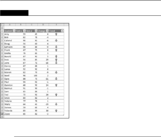
FIGURE 20.14

Hiding one of the icons makes the table less cluttered.

Creating Formula-Based Rules

Excel’s conditional formatting feature is versatile, but sometimes it’s just not quite versatile enough. Fortunately, you can extend its versatility by writing conditional formatting formulas.

The examples later in this section describe how to create conditional formatting formulas for the following:

•To identify text entries

•To identify dates that fall on a weekend

•To format cells that are in odd-numbered rows or columns (for dynamic alternate row or columns shading)

•To format groups of rows (for example, shade every two groups of rows)

•To display a sum only when all precedent cells contain values

Some of these formulas may be useful to you. If not, they may inspire you to create other conditional formatting formulas.

494

Chapter 20: Visualizing Data Using Conditional Formatting

On the CD

The companion CD-ROM contains all the examples in this section. The file is named conditional formatting formulas.xlsx.

To specify conditional formatting based on a formula, select the cells and then choose Home Styles Conditional Formatting New Rule. This command displays the New Formatting Rule dialog box. Click the rule type Use a Formula to Determine Which Cells to Format, and you can specify the formula.

You can type the formula directly into the box, or you can enter a reference to a cell that contains a logical formula. As with normal Excel formulas, the formula you enter here must begin with an equal sign (=).

Note

The formula must be a logical formula that returns either TRUE or FALSE. If the formula evaluates to TRUE, the condition is satisfied, and the conditional formatting is applied. If the formula evaluates to FALSE, the conditional formatting is not applied. n

Understanding relative and absolute references

If the formula that you enter into the Conditional Formatting dialog box contains a cell reference, that reference is considered a relative reference, based on the upper-left cell in the selected range.

For example, suppose that you want to set up a conditional formatting condition that applies shading to cells in range A1:B10 only if the cell contains text. None of Excel’s conditional formatting options can do this task, so you need to create a formula that will return TRUE if the cell contains text and FALSE otherwise. Follow these steps:

1.Select the range A1:B10 and ensure that cell A1 is the active cell.

2.Choose Home Styles Conditional Formatting New Rule to display the New

Formatting Rule dialog box.

3.Click the Use a Formula to Determine Which Cells to Format rule type.

4.Enter the following formula in the Formula box:

=ISTEXT(A1)

5.Click the Format button to display the Format Cells dialog box.

6.From the Fill tab, specify the cell shading that will be applied if the formula returns

TRUE.

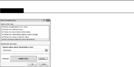
7.Click OK to return to the New Formatting Rule dialog box (see Figure 20.15).

8.In the New Formatting Rule dialog box, click the Preview button. Make sure that the formula is working correctly and to see a preview of your selected formatting.

9.If the preview looks correct, click OK to close the New Formatting Rule dialog box.

Notice that the formula entered in Step 4 contains a relative reference to the upper-left cell in the selected range.

495

Part III: Creating Charts and Graphics

FIGURE 20.15

Creating a conditional formatting rule based on a formula.

Generally, when entering a conditional formatting formula for a range of cells, you’ll use a reference to the active cell, which is typically the upper-left cell in the selected range. One exception is when you need to refer to a specific cell. For example, suppose that you select range A1:B10, and you want to apply formatting to all cells in the range that exceed the value in cell C1. Enter this conditional formatting formula:

=A1>$C$1

In this case, the reference to cell C1 is an absolute reference; it will not be adjusted for the cells in the selected range. In other words, the conditional formatting formula for cell A2 looks like this:

=A2>$C$1

The relative cell reference is adjusted, but the absolute cell reference is not.

Conditional formatting formula examples

Each of these examples uses a formula entered directly into the New Formatting Rule dialog box, after selecting the Use a Formula to Determine Which Cells to Format rule type. You decide the type of formatting that you apply conditionally.

Identifying weekend days

Excel provides a number of conditional formatting rules that deal with dates, but it doesn’t let you identify dates that fall on a weekend. Use this formula to identify weekend dates:

=OR(WEEKDAY(A1)=7,WEEKDAY(A1)=1)

This formula assumes that a range is selected and that cell A1 is the active cell.

496

Chapter 20: Visualizing Data Using Conditional Formatting

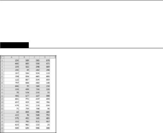
Displaying alternate-row shading

The conditional formatting formula that follows was applied to the range A1:D18, as shown in Figure 20.16, to apply shading to alternate rows.

=MOD(ROW(),2)=0

Alternate row shading can make your spreadsheets easier to read. If you add or delete rows within the conditional formatting area, the shading is updated automatically.

This formula uses the ROW function (which returns the row number) and the MOD function (which returns the remainder of its first argument divided by its second argument). For cells in even-numbered rows, the MOD function returns 0, and cells in that row are formatted.

For alternate shading of columns, use the COLUMN function instead of the ROW function.

FIGURE 20.16

Using conditional formatting to apply formatting to alternate rows.

Creating checkerboard shading

The following formula is a variation on the example in the preceding section. It applies formatting to alternate rows and columns, creating a checkerboard effect.

=MOD(ROW(),2)=MOD(COLUMN(),2)

Shading groups of rows

Here’s another rows shading variation. The following formula shades alternate groups of rows. It produces four rows of shaded rows, followed by four rows of unshaded rows, followed by four more shaded rows, and so on.

=MOD(INT((ROW()-1)/4)+1,2)

497

Part III: Creating Charts and Graphics

Figure 20.17 shows an example.

For different sized groups, change the 4 to some other value. For example, use this formula to shade alternate groups of two rows:

=MOD(INT((ROW()-1)/2)+1,2)

FIGURE 20.17

Conditional formatting produces these groups of alternate shaded rows.

Displaying a total only when all values are entered

Figure 20.18 shows a range with a formula that uses the SUM function in cell C6. Conditional formatting is used to hide the sum if any of the four cells above is blank. The conditional formatting formula for cell C6 (and cell C5, which contains a label) is

=COUNT($C$2:$C$5)=4

This formula returns TRUE only if C2:C5 contains no empty cells.

Figure 20.19 shows the worksheet when one of the values is missing.

498