Part II: Working with Formulas and Functions

Tip

If your worksheet uses any data tables (described in Chapter 36), you may want to select the Automatically Except for Data Tables option. Large data tables calculate notoriously slowly. Note: A data table is not the same as a table created by choosing Insert Tables Table. n

When you’re working in Manual Calculation mode, Excel displays Calculate in the status bar when you have any uncalculated formulas. You can use the following shortcut keys to recalculate the formulas:

•F9: Calculates the formulas in all open workbooks.

•Shift+F9: Calculates only the formulas in the active worksheet. Other worksheets in the same workbook aren’t calculated.

•Ctrl+Alt+F9: Forces a complete recalculation of all formulas.

Note

Excel’s Calculation mode isn’t specific to a particular worksheet. When you change the Calculation mode, it affects all open workbooks, not just the active workbook. n

Using Advanced Naming Techniques

Using range names can make your formulas easier to understand, easier to modify, and even help prevent errors. It’s much easier to deal with a meaningful name such as AnnualSales than with a range reference, such as AB12:AB68.

Cross-Reference

See Chapter 4 for basic information regarding working with names. n

Excel offers a number of advanced techniques that make using names even more useful. I discuss these techniques in the sections that follow.

Using names for constants

Many Excel users don’t realize that you can give a name to an item that doesn’t appear in a cell. For example, if formulas in your worksheet use a sales-tax rate, you would probably insert the tax-rate value into a cell and use this cell reference in your formulas. To make things easier, you would probably also name this cell something similar to SalesTax.

Here’s how to provide a name for a value that doesn’t appear in a cell:

1.Choose Formulas Defined Names Define Name. Excel displays the New Name dialog box.

2.Enter the name (in this case, SalesTax) into the Name field.

222

Chapter 10: Introducing Formulas and Functions

3.Select a scope in which the name will be valid (either the entire workbook or a specific worksheet).

4.Click the Refers To text box, delete its contents, and replace the old contents with a value (such as .075).

5.(Optional). Use the Comment box to provide a comment about the name.

6.Click OK to close the New Name dialog box and create the name.

You just created a name that refers to a constant rather than a cell or range. Now if you type =SalesTax into a cell that’s within the scope of the name, this simple formula returns 0.075 — the constant that you defined. You also can use this constant in a formula, such as

=A1*SalesTax.

Tip

A constant also can be text. For example, you can define a constant for your company’s name. n

Note

Named constants don’t appear in the Name box or in the Go To dialog box. This makes sense because these constants don’t reside anywhere tangible. They do appear in the drop-down list that’s displayed when you enter a formula — which is handy because you use these names in formulas. n

Using names for formulas

Just like you can create a named constant, you can also create named formulas. Like with named constants, named formulas don’t appear in the worksheet.

You create named formulas the same way you create named constants — by using the New Name dialog box. For example, you might create a named formula that calculates the monthly interest rate from an annual rate; Figure 10.16 shows an example. In this case, the name MonthlyRate refers to the following formula:

=Sheet3!$B$1/12

FIGURE 10.16

Excel allows you to name a formula that doesn’t exist in a worksheet cell.

223

Part II: Working with Formulas and Functions

When you use the name MonthlyRate in a formula, it uses the value in B1 divided by 12. Notice that the cell reference is an absolute reference.

Naming formulas gets more interesting when you use relative references rather than absolute references. When you use the pointing technique to create a formula in the Refers To field of the New Name dialog box, Excel always uses absolute cell references — which is unlike its behavior when you create a formula in a cell.

For example, activate cell B1 on Sheet1 and create the name Cubed for the following formula:

=Sheet1!A1^3

In this example, the relative reference points to the cell to the left of the cell in which the name is used. Therefore, make certain that cell B1 is the active cell before you open the New Name dialog box; this is very important. The formula contains a relative reference; when you use this named formula in a worksheet, the cell reference is always relative to the cell that contains the formula. For example, if you enter =Cubed into cell D12, then cell D12 displays the contents of cell C12 raised to the third power (C12 is the cell directly to the left of D12).

Using range intersections

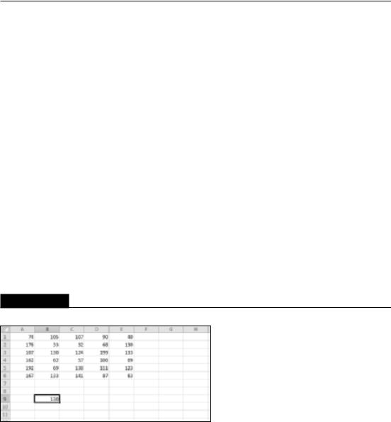
This section describes a concept known as range intersections — individual cells that two ranges have in common. Excel uses an intersection operator — a space character — to determine the overlapping references in two ranges. Figure 10.17 shows a simple example.

FIGURE 10.17

You can use a range-intersection formula to determine values.

The formula in cell B9 is

=B1:B6 A3:D3

This formula returns 130, the value in cell B3 — that is, the value at the intersection of the two ranges.

224

Chapter 10: Introducing Formulas and Functions

The intersection operator is one of three reference operators used with ranges. Table 10.4 lists these operators.

TABLE 10.4

The real value of knowing about range intersections is apparent when you use names. Examine Figure 10.18, which shows a table of values. I selected the entire table and then used Formulas Defined Names Create from Selection to create names automatically by using the top row and left column.

FIGURE 10.18

When you use names, using a range-intersection formula to determine values is even more useful.

Excel created the following names:

With these names defined, you can create formulas that are easy to read and use. For example, to calculate the total for Quarter 4, just use this formula:

=SUM(Quarter4)

225

Part II: Working with Formulas and Functions

To refer to a single cell, use the intersection operator. Move to any blank cell and enter the following formula:

=Quarter1 West

This formula returns the value for the first quarter for the West region. In other words, it returns the value that exists where the Quarter1 range intersects with the West range. Naming ranges in this manner can help you create very readable formulas.

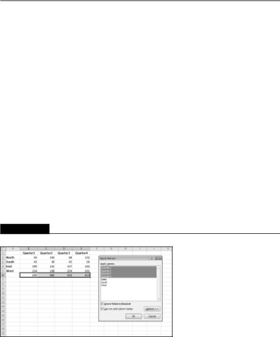
Applying names to existing references

When you create a name for a cell or a range, Excel doesn’t automatically use the name in place of existing references in your formulas. For example, suppose you have the following formula in cell F10:

=A1–A2

If you define a name Income for A1 and Expenses for A2, Excel won’t automatically change your formula to =Income–Expenses. Replacing cell or range references with their corresponding names is fairly easy, however.

To apply names to cell references in formulas after the fact, start by selecting the range that you want to modify. Then choose Formulas Defined Names Define Name Apply Names. Excel displays the Apply Names dialog box, as shown in Figure 10.19. Select the names that you want to apply by clicking them and then click OK. Excel replaces the range references with the names in the selected cells.

FIGURE 10.19

Use the Apply Names dialog box to replace cell or range references with defined names.

226