Chapter 11: Creating Formulas That Manipulate Text

For example, assume that cell A1 contains the text Annual Profit Figures. The following formula searches for the six-letter word Profit and replaces it with the word Loss:

=REPLACE(A1,SEARCH(“Profit”,A1),6,”Loss”)

This next formula uses the SUBSTITUTE function to accomplish the same effect in a more efficient manner:

=SUBSTITUTE(A1,”Profit”,”Loss”)

Advanced Text Formulas

The examples in this section appear more complex than the examples in the preceding section. As you can see, though, these examples can perform some very useful text manipulations. Space limitations prevent a detailed explanation of how these formulas work, but this section gives you a basic introduction.

On the CD

You can access all the examples in this section on the companion CD-ROM. The file is named text formula examples.xlsx.

Counting specific characters in a cell

This formula counts the number of Bs (uppercase only) in the string in cell A1:

=LEN(A1)-LEN(SUBSTITUTE(A1,”B”,””))

This formula works by using the SUBSTITUTE function to create a new string (in memory) that has all the Bs removed. Then the length of this string is subtracted from the length of the original string. The result reveals the number of Bs in the original string.

The following formula is a bit more versatile: It counts the number of Bs (both uppercase and lowercase) in the string in cell A1. Using the UPPER function to convert the string makes this formula work with both uppercase and lowercase characters:

=LEN(A1)-LEN(SUBSTITUTE(UPPER(A1),”B”,””))

Counting the occurrences of a substring in a cell

The formulas in the preceding section count the number of occurrences of a particular character in a string. The following formula works with more than one character. It returns the number of occurrences of a particular substring (contained in cell B1) within a string (contained in cell A1). The substring can consist of any number of characters.

=(LEN(A1)-LEN(SUBSTITUTE(A1,B1,””)))/LEN(B1)

243

Part II: Working with Formulas and Functions

For example, if cell A1 contains the text Blonde On Blonde and B1 contains the text Blonde, the formula returns 2.

The comparison is case sensitive, so if B1 contains the text blonde, the formula returns 0. The following formula is a modified version that performs a case-insensitive comparison by converting the characters to uppercase:

=(LEN(A1)-LEN(SUBSTITUTE(UPPER(A1),UPPER(B1),””)))/LEN(B1)

Extracting a filename from a path specification

The following formula returns the filename from a full path specification. For example, if cell A1 contains c:\windows\important\myfile.xlsx, the formula returns myfile.xlsx.

=MID(A1,FIND(“*”,SUBSTITUTE(A1,”\”,”*”,LEN(A1)-LEN(SUBSTITUTE(A1,”\”, ””))))+1,LEN(A1))

This formula assumes that the system path separator is a backslash (\). It essentially returns all text that follows the last backslash character. If cell A1 doesn’t contain a backslash character, the formula returns an error.

Extracting the first word of a string

To extract the first word of a string, a formula must locate the position of the first space character and then use this information as an argument for the LEFT function. The following formula does just that:

=LEFT(A1,FIND(“ “,A1)-1)

This formula returns all the text prior to the first space in cell A1. However, the formula has a slight problem: It returns an error if cell A1 consists of a single word. A slightly more complex formula that checks for the error using the IFERROR function solves that problem:

=IFERROR(LEFT(A1,FIND(“ “,A1)-1),A1)

Caution

The preceding formula uses the IFERROR function, which was introduced in Excel 2007. If your workbook will be used with previous versions of Excel, use this formula:

=IF(ISERR(FIND(“ “,A1)),A1,LEFT(A1,FIND(“ “,A1)-1))

Extracting the last word of a string

Extracting the last word of a string is more complicated because the FIND function only works from left to right. Therefore the problem is locating the last space character. The formula that follows, however, solves this problem by returning the last word of a string (all text following the last space character):

244

Chapter 11: Creating Formulas That Manipulate Text

=RIGHT(A1,LEN(A1)-FIND(“*”,SUBSTITUTE(A1,” “,”*”,LEN(A1)- LEN(SUBSTITUTE(A1,” “,””)))))

This formula, however, has the same problem as the first formula in the preceding section: It fails if the string does not contain at least one space character. The following modified formula uses the IFERROR function to test for an error (that is, no spaces). If the first argument returns an error, the formula returns the complete contents of cell A1:

=IFERROR(RIGHT(A1,LEN(A1)-FIND(“*”,SUBSTITUTE(A1,” “,”*”,LEN(A1)- LEN(SUBSTITUTE(A1,” “,””))))),A1)

Following is a modification that doesn’t use the IFERROR function. This formula works for all versions of Excel:

=IF(ISERR(FIND(“ “,A1)),A1,RIGHT(A1,LEN(A1)-FIND(“*”,SUBSTITUTE(A1,” “,”*”,LEN(A1)-LEN(SUBSTITUTE(A1,” “,””))))))

Extracting all but the first word of a string

The following formula returns the contents of cell A1, except for the first word:

=RIGHT(A1,LEN(A1)-FIND(“ “,A1,1))

If cell A1 contains 2010 Operating Budget, the formula returns Operating Budget.

The following formula, which uses the IFERROR function, returns the entire contents of cell A1 if the cell doesn’t have a space character:

=IFERROR(RIGHT(A1,LEN(A1)-FIND(“ “,A1,1)),A1)

A modification that works in all versions of Excel is

=IF(ISERR(FIND(“ “,A1)),A1,RIGHT(A1,LEN(A1)-FIND(“ “,A1,1)))

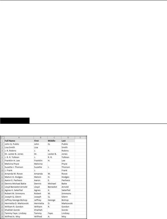
Extracting first names, middle names, and last names

Suppose you have a list consisting of people’s names in a single column. You have to separate these names into three columns: one for the first name, one for the middle name or initial, and one for the last name. This task is more complicated than you may think because it must handle the situation for a missing middle initial. However, you can still do it.

Note

The task becomes a lot more complicated if the list contains names with titles (such as Mr. or Dr.) or names followed by additional details (such as Jr. or III). In fact, the following formulas will not handle these complex cases. However, they still give you a significant head start if you’re willing to do a bit of manual editing to handle special cases. For a way to remove these titles, see the next section, “Removing titles from names.” n

245

Part II: Working with Formulas and Functions

The formulas that follow all assume that the name appears in cell A1.

You can easily construct a formula to return the first name:

=LEFT(A1,FIND(“ “,A1)-1)

This formula returns the last name:

=RIGHT(A1,LEN(A1)-FIND(“*”,SUBSTITUTE(A1,” “,”*”,LEN(A1)- LEN(SUBSTITUTE(A1,” “,””)))))

The next formula extracts the middle name and requires that you use the other formulas to extract the first name and the last name. It assumes that the first name is in B1 and the last name is in D1. Here’s what it looks like:

=IF(LEN(B1&D1)+2>=LEN(A1),””,MID(A1,LEN(B1)+2,LEN(A1)-LEN(B1&D1)-2))

As you can see in Figure 11.5, the formulas work fairly well. There are a few problems, however, notably names that contain four “words.” But, as I mentioned earlier, you can clean up these cases manually.

On the CD

This workbook, named extract names.xlsx, is available on the companion CD-ROM. n

FIGURE 11.5

This worksheet uses formulas to extract the first name, last name, and middle name (or initial) from a list of names in column A.

246

Chapter 11: Creating Formulas That Manipulate Text

Splitting Text Strings without Using Formulas

In many cases, you can eliminate the use of formulas and use the Text to Columns command to parse strings into their component parts. This command is found in the Data Tools group of the Data tab. Text to Columns displays the Convert Text to Columns Wizard, which consists of a series of dialog boxes that walk you through the steps to convert a single column of data into multiple columns. Generally, you want to select the Delimited option (in Step 1) and use Space as the delimiter (in Step 2), as shown in the following figure.

Removing titles from names

You can use the formula that follows to remove three common titles (Mr., Ms., and Mrs.) from a name. For example, if cell A1 contains Mr. Fred Munster, the formula would return Fred Munster.

=IF(OR(LEFT(A1,2)=”Mr”,LEFT(A1,3)=”Mrs”,LEFT(A1,2)=”Ms”), RIGHT(A1,LEN(A1) -FIND(“ “,A1)),A1)

Creating an ordinal number

An ordinal number is an adjective form of a number. Examples include 1st, 2nd, 5th, 23rd, and so on. The formula that follows displays the value in cell A1 as an ordinal number:

=A13&IF(OR(VALUE(RIGHT(A1,2))={11,12,13}),”th”,

IF(OR(VALUE(RIGHT(A1))={1,2,3}),CHOOSE(RIGHT(A1),

“st”,”nd”,”rd”),”th”))

247

Part II: Working with Formulas and Functions

The formula is rather complex because it must determine whether the number will end in th, st, nd, or rd. This formula also uses literal arrays (enclosed in brackets), which are described in Chapter 17.

Counting the number of words in a cell

The following formula returns the number of words in cell A1:

=LEN(TRIM(A1))-LEN(SUBSTITUTE( (A1),” “,””))+1

The formula uses the TRIM function to remove excess spaces. It then uses the SUBSTITUTE function to create a new string (in memory) that has all the space characters removed. The length of this string is subtracted from the length of the original (trimmed) string to get the number of spaces. This value is then incremented by 1 to get the number of words.

Note that this formula will return 1 if the cell is empty. The following modification solves that problem:

=IF(LEN(A1)=0,0,LEN(TRIM(A1))-LEN(SUBSTITUTE(TRIM(A1),” “,””))+1)

248

CHAPTER

Working with Dates and Times

249

Part II: Working with Formulas and Functions

A serial number of 1 corresponds to January 1, 1900; a serial number of 2 corresponds to January 2, 1900, and so on. This system makes it possible to deal with dates in formulas. For example, you can create a formula to calculate the number of days between two dates (just subtract one from the other).

Excel support dates from January 1, 1900, through December 31, 9999 (serial number = 2,958,465).

You may wonder about January 0, 1900. This nondate (which corresponds to date serial number 0) is actually used to represent times that aren’t associated with a particular day. This concept becomes clear later in this chapter (see “Entering times”).

To view a date serial number as a date, you must format the cell as a date. Choose Home Number Number Format. This drop-down control provides you with two date formats. To select from additional date formats, see “Formatting dates and times,” later in this chapter.

Entering dates

You can enter a date directly as a serial number (if you know the serial number) and then format it as a date. More often, you enter a date by using any of several recognized date formats. Excel automatically converts your entry into the corresponding date serial number (which it uses for calculations), and it also applies the default date format to the cell so that it displays as an actual date rather than as a cryptic serial number.

Choose Your Date System: 1900 or 1904

Excel supports two date systems: the 1900 date system and the 1904 date system. Which system you use in a workbook determines what date serves as the basis for dates. The 1900 date system uses January 1, 1900 as the day assigned to date serial number 1. The 1904 date system uses January 1, 1904, as the base date. By default, Excel for Windows uses the 1900 date system, and Excel for Macintosh uses the 1904 date system. Excel for Windows supports the 1904 date system for compatibility with Macintosh files. You can choose the date system for the active workbook in the Advanced section of the Excel Options dialog box. (It’s in the When Calculating This Workbook subsection.) You can’t change the date system if you use Excel for Macintosh.

Generally, you should use the default 1900 date system. And you should exercise caution if you use two different date systems in workbooks that are linked. For example, assume that Book1 uses the 1904 date system and contains the date 1/15/1999 in cell A1. Assume that Book2 uses the 1900 date system and contains a link to cell A1 in Book1. Book2 displays the date as 1/14/1995. Both workbooks use the same date serial number (34713), but they’re interpreted differently.

One advantage to using the 1904 date system is that it enables you to display negative time values. With the 1900 date system, a calculation that results in a negative time (for example, 4:00 PM–5:30 PM) cannot be displayed. When using the 1904 date system, the negative time displays as –1:30 (that is, a difference of 1 hour and 30 minutes).

250

Chapter 12: Working with Dates and Times

For example, if you need to enter June 18, 2010 into a cell, you can enter the date by typing June 18, 2010 (or any of several different date formats). Excel interprets your entry and stores the value 40347, the date serial number for that date. It also applies the default date format, so the cell contents may not appear exactly as you typed them.

Note

Depending on your regional settings, entering a date in a format such as June 18, 2010 may be interpreted as a text string. In such a case, you need to enter the date in a format that corresponds to your regional settings, such as 18 June, 2010. n

When you activate a cell that contains a date, the Formula bar shows the cell contents formatted by using the default date format — which corresponds to your system’s short date format. The Formula bar doesn’t display the date’s serial number. If you need to find out the serial number for a particular date, format the cell with a nondate number format.

Tip

To change the default date format, you need to change a system-wide setting. From the Windows Control Panel, select Regional and Language Options. The exact procedure varies, depending on the version of Windows you use. Look for the drop-down list that enables you to change the Short Date Format. The setting you choose determines the default date format that Excel uses to display dates in the Formula bar. n

Table 12.1 shows a sampling of the date formats that Excel recognizes (using the U.S. settings). Results will vary if you use a different regional setting.

TABLE 12.1

251

Part II: Working with Formulas and Functions

Searching for Dates

If your worksheet uses many dates, you may need to search for a particular date by using the Find and Replace dialog box (Home Editing Find & Select Find, or Ctrl+F). Excel is rather picky when it comes to finding dates. You must enter the date as it appears in the formula bar. For example, if a cell contains a date formatted to display as June 19, 2010, the date appears in the Formula bar using your system’s short date format (for example, 6/19/2010). Therefore, if you search for the date as it appears in the cell, Excel won’t find it. But it will find the cell if you search for date in the format that appears in the Formula bar.

As you can see in Table 12.1, Excel is rather flexible when it comes to recognizing dates entered into a cell. It’s not perfect, however. For example, Excel does not recognize any of the following entries as dates:

•June 18 2010

•Jun-18 2010

•Jun-18/2010

Rather, it interprets these entries as text. If you plan to use dates in formulas, make sure that Excel can recognize the date you enter as a date; otherwise, the formulas that refer to these dates will produce incorrect results.

If you attempt to enter a date that lies outside of the supported date range, Excel interprets it as text. If you attempt to format a serial number that lies outside of the supported range as a date, the value displays as a series of hash marks (#########).

Understanding time serial numbers

When you need to work with time values, you extend the Excel date serial number system to include decimals. In other words, Excel works with times by using fractional days. For example, the date serial number for June 1, 2010 is 40330. Noon (halfway through the day) is represented internally as 40330.5.

The serial number equivalent of one minute is approximately 0.00069444. The formula that follows calculates this number by multiplying 24 hours by 60 minutes, and dividing the result into 1. The denominator consists of the number of minutes in a day (1,440).

=1/(24*60)

Similarly, the serial number equivalent of one second is approximately 0.00001157, obtained by the following formula:

1 / 24 hours × 60 minutes × 60 seconds

In this case, the denominator represents the number of seconds in a day (86,400).

=1/(24*60*60)

252

Chapter 12: Working with Dates and Times

In Excel, the smallest unit of time is one one-thousandth of a second. The time serial number shown here represents 23:59:59.999 (one one-thousandth of a second before midnight):

0.99999999

Table 12.2 shows various times of day along with each associated time serial numbers.

TABLE 12.2

Times of Day and Their Corresponding Serial Numbers

Entering times

As with entering dates, you normally don’t have to worry about the actual time serial numbers. Just enter the time into a cell using a recognized format. Table 12.3 shows some examples of time formats that Excel recognizes.

TABLE 12.3

253

Part II: Working with Formulas and Functions

Because the preceding samples don’t have a specific day associated with them, Excel (by default) uses a date serial number of 0, which corresponds to the nonday January 0, 1900. Often, you’ll want to combine a date and time. Do so by using a recognized date-entry format, followed by a space, and then a recognized time-entry format. For example, if you enter 6/18/2010 11:30 in a cell, Excel interprets it as 11:30 a.m. on June 18, 2010. Its date/time serial number is 40347.479166667.

When you enter a time that exceeds 24 hours, the associated date for the time increments accordingly. For example, if you enter 25:00:00 into a cell, it’s interpreted as 1:00 a.m. on January 1, 1900. The day part of the entry increments because the time exceeds 24 hours. Keep in mind that a time value without a date uses January 0, 1900 as the date.

Similarly, if you enter a date and a time (and the time exceeds 24 hours), the date that you entered is adjusted. If you enter 9/18/2010 25:00:00, for example, it’s interpreted as 9/19/2010 1:00:00 a.m.

If you enter a time only (without an associated date) into an unformatted cell, the maximum time that you can enter into a cell is 9999:59:59 (just less than 10,000 hours). Excel adds the appropriate number of days. In this case, 9999:59:59 is interpreted as 3:59:59 p.m. on 02/19/1901. If you enter a time that exceeds 10,000 hours, the entry is interpreted as a text string rather than a time.

Formatting dates and times

You have a great deal of flexibility in formatting cells that contain dates and times. For example, you can format the cell to display the date part only, the time part only, or both the date and time parts.

You format dates and times by selecting the cells and then using the Number tab of the Format Cells dialog box, as shown in Figure 12.1. To display this dialog box, click the dialog box launcher icon in the Number group of the Home tab. Or, click Number Format and choose More Number Formats from the list that appears.

The Date category shows built-in date formats, and the Time category shows built-in time formats. Some formats include both date and time displays. Just select the desired format from the Type list and then click OK.

Tip

When you create a formula that refers to a cell containing a date or a time, Excel sometimes automatically formats the formula cell as a date or a time. Often, this automation is very helpful; other times, it’s completely inappropriate and downright annoying. To return the number formatting to the default General format, choose Home Number Number Format and choose General from the drop-down list. Or, press Ctrl+Shift+~. n

If none of the built-in formats meets your needs, you can create a custom number format. Select the Custom category and then type the custom format codes into the Type box. (See Chapter 24 for information on creating custom number formats.)

254

Chapter 12: Working with Dates and Times

FIGURE 12.1

Use the Number tab in the Format Cells dialog box to change the appearance of dates and times.

Problems with dates

Excel has some problems when it comes to dates. Many of these problems stem from the fact that Excel was designed many years ago. Excel designers basically emulated the Lotus 1-2-3 program’s limited date and time features, which contain a nasty bug that was duplicated intentionally in Excel. (You can read why in a bit.) If Excel were being designed from scratch today, I’m sure it would be much more versatile in dealing with dates. Unfortunately, users are currently stuck with a product that leaves much to be desired in the area of dates.

Excel’s leap year bug

A leap year, which occurs every four years, contains an additional day (February 29). Specifically, years that are evenly divisible by 100 are not leap years, unless they are also evenly divisible by 400. Although the year 1900 was not a leap year, Excel treats it as such. In other words, when you type 2/29/1900 into a cell, Excel interprets it as a valid date and assigns a serial number of 60.

If you type 2/29/1901, however, Excel correctly interprets it as a mistake and doesn’t convert it to a date. Rather, it simply makes the cell entry a text string.

How can a product used daily by millions of people contain such an obvious bug? The answer is historical. The original version of Lotus 1-2-3 contained a bug that caused it to treat 1900 as a leap year. When Excel was released some time later, the designers knew of this bug and chose to reproduce it in Excel to maintain compatibility with Lotus worksheet files.

255

Part II: Working with Formulas and Functions

Why does this bug still exist in later versions of Excel? Microsoft asserts that the disadvantages of correcting this bug outweigh the advantages. If the bug were eliminated, it would mess up millions of existing workbooks. In addition, correcting this problem would possibly affect compatibility between Excel and other programs that use dates. As it stands, this bug really causes very few problems because most users don’t use dates prior to March 1, 1900.

Pre-1900 dates

The world, of course, didn’t begin on January 1, 1900. People who use Excel to work with historical information often need to work with dates before January 1, 1900. Unfortunately, the only way to work with pre-1900 dates is to enter the date into a cell as text. For example, you can enter July 4, 1776 into a cell, and Excel won’t complain.

Tip

If you plan to sort information by old dates, you should enter your text dates with a four-digit year, followed by a two-digit month, and then a two-digit day: for example, 1776-07-04. This format will enable accurate sorting. n

Using text as dates works in some situation, but the main problem is that you can’t perform any manipulation on a date that’s entered as text. For example, you can’t change its numeric formatting, you can’t determine which day of the week this date occurred on, and you can’t calculate the date that occurs seven days later.

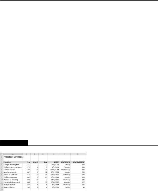
On the CD

The companion CD-ROM contains a workbook named XDATE demo.xlsm. This workbook contains eight custom worksheet functions written in VBA. These functions enable you to work with any date in the years 0100 through 9999. Figure 12.2 shows a worksheet that uses these extended date functions in columns E though G to perform calculations that involve pre-1900 dates.

FIGURE 12.2

The author’s Extended Date Functions add-in enables you to work with pre-1900 dates.

256

Chapter 12: Working with Dates and Times

Inconsistent date entries

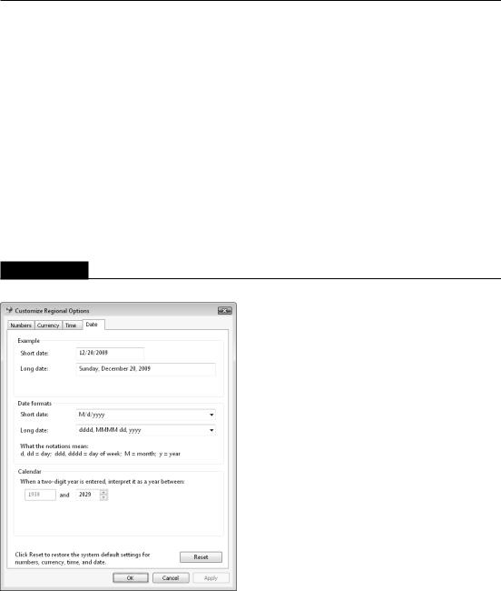
You need to exercise caution when entering dates by using two digits for the year. When you do so, Excel has some rules that kick in to determine which century to use. And those rules vary, depending on the version of Excel that you use.

Two-digit years between 00 and 29 are interpreted as 21st century dates, and two-digit years between 30 and 99 are interpreted as 20th-century dates. For example, if you enter 12/15/28, Excel interprets your entry as December 15, 2028. But if you enter 12/15/30, Excel sees it as December 15, 1930 because Windows uses a default boundary year of 2029. You can keep the default as is or change it via the Windows Control Panel. From the Regional and Language Options dialog box, click the Customize button to display the Customize Regional Options dialog box. Select the Date tab and then specify a different year.

Figure 12.3 shows this dialog box in Windows Vista. This procedure may vary with different versions of Windows.

FIGURE 12.3

Use the Windows Control Panel to specify how Excel interprets two-digit years.

Tip

The best way to avoid any surprises is to simply enter all years using all four digits for the year. n

257