CHAPTER

Creating Formulas

That Look Up Values

Note

I use the term table to describe a rectangular range of data. The range does not necessarily need to be an “official” table, as created by choosing Insert Tables Table. n

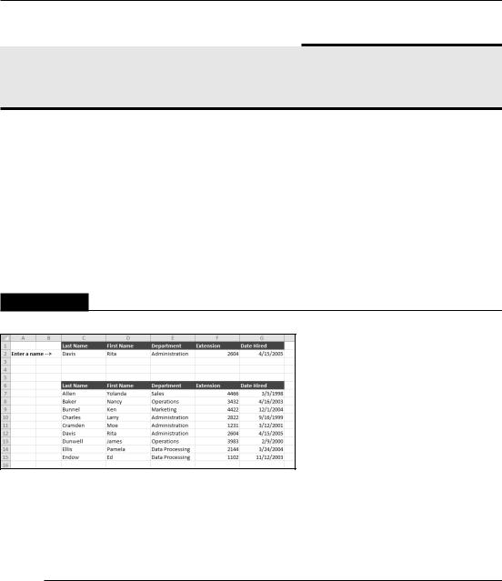
Figure 14.1 shows a worksheet that uses several lookup formulas. This worksheet contains a table of employee data, beginning in row 7. This range is named EmpData. When you enter a last name into cell C2, lookup formulas in D2:G2 retrieve the matching information from the table. If the last name does not appear in Column C, the formulas return #N/A.

309

Part II: Working with Formulas and Functions

About This Chapter’s Examples

Most of the examples in this chapter use named ranges for function arguments. When you adapt these formulas for your own use, you need to substitute the actual range address or a range name defined in your workbook.

FIGURE 14.1

Lookup formulas in row 2 look up the information for the employee name in cell C2.

This particular example uses four formulas to return information from the EmpData range. In many cases, you want only a single value from the table, so use only one formula.

Functions Relevant to Lookups

Several Excel functions are useful when writing formulas to look up information in a table. Table 14.1 lists and describes these functions.

310

Chapter 14: Creating Formulas That Look Up Values

TABLE 14.1

* Introduced in Excel 2007.

The examples in this chapter use the functions listed in Table 14.1.

Using the IF Function for Simple Lookups

The IF function is very versatile and is often suitable for simple decision-making problems. The accompanying figure shows a worksheet with student grades in column B. Formulas in column C use the IF function to return text: either Pass (a score of 65 or higher) or Fail (a score below 65). For example, the formula in cell C2 is

=IF(B2>=65,”Pass”,”Fail”)

continued

311

Part II: Working with Formulas and Functions

continued

You can “nest” IF functions to provide even more decision-making ability. This formula, for example, returns one of four strings: Excellent, Very Good, Fair, or Poor.

=IF(B2>=90,”Excellent”,IF(B2>=70,”Very Good”,IF(B2>=50,”Fair”,”Poor”)))

This technique is fine for situations that involve only a few choices. However, using nested IF functions can quickly become complicated and unwieldy. The lookup techniques described in this chapter usually provide a much better solution.

Basic Lookup Formulas

You can use the Excel basic lookup functions to search a column or row for a lookup value to return another value as a result. Excel provides three basic lookup functions: HLOOKUP, VLOOKUP, and LOOKUP. In addition, the MATCH and INDEX functions are often used together to return a cell or relative cell reference for a lookup value.

The VLOOKUP function

The VLOOKUP function looks up the value in the first column of the lookup table and returns the corresponding value in a specified table column. The lookup table is arranged vertically (which explains the V in the function’s name). The syntax for the VLOOKUP function is

VLOOKUP(lookup_value,table_array,col_index_num,range_lookup)

The VLOOKUP function’s arguments are as follows:

•lookup_value: The value to be looked up in the first column of the lookup table.

•table_array: The range that contains the lookup table.

•col_index_num: The column number within the table from which the matching value is returned.

•range_lookup: Optional. If TRUE or omitted, an approximate match is returned. (If an exact match is not found, the next largest value that is less than lookup_value is returned.) If FALSE, VLOOKUP will search for an exact match. If VLOOKUP can’t find an exact match, the function returns #N/A.

Caution

If the range_lookup argument is TRUE or omitted, the first column of the lookup table must be in ascending order. If lookup_value is smaller than the smallest value in the first column of table_array, VLOOKUP returns #N/A. If the range_lookup argument is FALSE, the first column of the lookup table need not be in ascending order. If an exact match is not found, the function returns #N/A.

312

Chapter 14: Creating Formulas That Look Up Values

Tip

If the lookup_value argument is text and the range_lookup argument is False, the lookup_value can include wildcard characters * and ?.

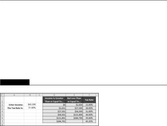
A very common use for a lookup formula involves an income tax rate schedule (see Figure 14.2). The tax rate schedule shows the income tax rates for various income levels. The following formula (in cell B3) returns the tax rate for the income in cell B2:

=VLOOKUP(B2,D2:F7,3)

On the CD

The examples in this section are available on the companion CD-ROM. They’re contained in a file named basic lookup examples.xlsx.

FIGURE 14.2

Using VLOOKUP to look up a tax rate.

The lookup table resides in a range that consists of three columns (D2:F7). Because the last argument for the VLOOKUP function is 3, the formula returns the corresponding value in the third column of the lookup table.

Note that an exact match is not required. If an exact match is not found in the first column of the lookup table, the VLOOKUP function uses the next largest value that is less than the lookup value. In other words, the function uses the row in which the value you want to look up is greater than or equal to the row value but less than the value in the next row. In the case of a tax table, this is exactly what you want to happen.

The HLOOKUP function

The HLOOKUP function works just like the VLOOKUP function except that the lookup table is arranged horizontally instead of vertically. The HLOOKUP function looks up the value in the first row of the lookup table and returns the corresponding value in a specified table row.

313

Part II: Working with Formulas and Functions

The syntax for the HLOOKUP function is

HLOOKUP(lookup_value,table_array,row_index_num,range_lookup)

The HLOOKUP function’s arguments are as follows

•lookup_value: The value to be looked up in the first row of the lookup table.

•table_array: The range that contains the lookup table.

•row_index_num: The row number within the table from which the matching value is returned.

•range_lookup: Optional. If TRUE or omitted, an approximate match is returned. (If an exact match is not found, the next largest value less than lookup_value is returned.) If FALSE, VLOOKUP will search for an exact match. If VLOOKUP can’t find an exact match, the function returns #N/A.

Tip

If the lookup_value argument is text and the range_lookup argument is False, the lookup_value can include wildcard characters * and?.

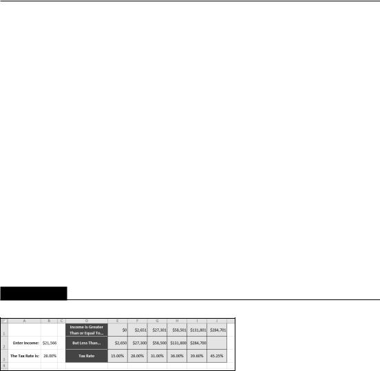
Figure 14.3 shows the tax rate example with a horizontal lookup table (in the range E1:J3). The formula in cell B3 is

=HLOOKUP(B2,E1:J3,3)

FIGURE 14.3

Using HLOOKUP to look up a tax rate.

The LOOKUP function

The LOOKUP function looks in a one-row or one-column range (lookup_vector) for a value (lookup_ value) and returns a value from the same position in a second one-row or one-column range (result_vector).

The LOOKUP function has the following syntax:

LOOKUP(lookup_value,lookup_vector,result_vector)

314

Chapter 14: Creating Formulas That Look Up Values

The function’s arguments are as follows:

•lookup_value: The value to be looked up in the lookup_vector.

•lookup_vector: A single-column or single-row range that contains the values to be looked up. These values must be in ascending order.

•result_vector: The single-column or single-row range that contains the values to be returned. It must be the same size as the lookup_vector.

Caution

Values in the lookup_vector must be in ascending order. If lookup_value is smaller than the smallest value in lookup_vector, LOOKUP returns #N/A.

Figure 14.4 shows the tax table again. This time, the formula in cell B3 uses the LOOKUP function to return the corresponding tax rate. The formula in cell B3 is

=LOOKUP(B2,D2:D7,F2:F7)

Caution

If the values in the first column are not arranged in ascending order, the LOOKUP function may return an incorrect value. n

Note that LOOKUP (as opposed to VLOOKUP) requires two range references (a range to be looked in, and a range that contains result values). VLOOKUP, on the other hand, uses a single range for the lookup table, and the third argument determines which column to use for the result. This argument, of course, can consist of a cell reference.

FIGURE 14.4

Using LOOKUP to look up a tax rate.

315

Part II: Working with Formulas and Functions

Combining the MATCH and INDEX functions

The MATCH and INDEX functions are often used together to perform lookups. The MATCH function returns the relative position of a cell in a range that matches a specified value. The syntax for

MATCH is

MATCH(lookup_value,lookup_array,match_type)

The MATCH function’s arguments are as follows:

•lookup_value: The value you want to match in lookup_array. If match_type is 0 and the lookup_value is text, this argument can include wildcard characters * and ?

•lookup_array: The range being searched.

•match_type: An integer (–1, 0, or 1) that specifies how the match is determined.

Note

If match_type is 1, MATCH finds the largest value less than or equal to lookup_value. (lookup_array must be in ascending order.) If match_type is 0, MATCH finds the first value exactly equal to lookup_value. If match_type is –1, MATCH finds the smallest value greater than or equal to lookup_value. (lookup_array must be in descending order.) If you omit the match_type argument, this argument is assumed to be 1.

The INDEX function returns a cell from a range. The syntax for the INDEX function is

INDEX(array,row_num,column_num)

The INDEX function’s arguments are as follows:

•array: A range

•row_num: A row number within array

•col_num: A column number within array

Note

If array contains only one row or column, the corresponding row_num or column_num argument is optional. n

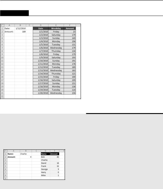
Figure 14.5 shows a worksheet with dates, day names, and amounts in columns D, E, and F. When you enter a date in cell B1, the following formula (in cell B2) searches the dates in column D and returns the corresponding amount from column F. The formula in cell B2 is

=INDEX(F2:F21,MATCH(B1,D2:D21,0))

To understand how this formula works, start with the MATCH function. This function searches the range D2:D21 for the date in cell B1. It returns the relative row number where the date is found. This value is then used as the second argument for the INDEX function. The result is the corresponding value in F2:F21.

316

Chapter 14: Creating Formulas That Look Up Values

FIGURE 14.5

Using the INDEX and MATCH functions to perform a lookup.

When a Blank Is Not a Zero

The Excel lookup functions treat empty cells in the result range as zeros. The worksheet in the accompanying figure contains a two-column lookup table, and this formula looks up the name in cell B1 and returns the corresponding amount:

=VLOOKUP(B1,D2:E8,2)

Note that the Amount cell for Charlie is blank, but the formula returns a 0.

continued

317