Part II: Working with Formulas and Functions

continued

If you need to distinguish zeros from blank cells, you must modify the lookup formula by adding an IF function to check whether the length of the returned value is 0. When the looked up value is blank, the length of the return value is 0. In all other cases, the length of the returned value is non-zero. The following formula displays an empty string (a blank) whenever the length of the looked-up value is zero and the actual value whenever the length is anything but zero:

=IF(LEN(VLOOKUP(B1,D2:E8,2))=0,””,(VLOOKUP(B1,D2:E8,2)))

Alternatively, you can specifically check for an empty string, as in the following formula:

=IF(VLOOKUP(B1,D2:E8,2)=””,””,(VLOOKUP(B1,D2:E8,2)))

Specialized Lookup Formulas

You can use additional types of lookup formulas to perform more specialized lookups. For example, you can look up an exact value, search in another column besides the first in a lookup table, perform a case-sensitive lookup, return a value from among multiple lookup tables, and perform other specialized and complex lookups.

On the CD

The examples in this section are available on the companion CD-ROM. The file is named specialized lookup examples.xlsx.

Looking up an exact value

As demonstrated in the previous examples, VLOOKUP and HLOOKUP don’t necessarily require an exact match between the value to be looked up and the values in the lookup table. An example is looking up a tax rate in a tax table. In some cases, you may require a perfect match. For example, when looking up an employee number, you would require a perfect match for the number.

To look up an exact value only, use the VLOOKUP (or HLOOKUP) function with the optional fourth argument set to FALSE.

Figure 14.6 shows a worksheet with a lookup table that contains employee numbers (column C) and employee names (column D). The lookup table is named EmpList. The formula in cell B2, which follows, looks up the employee number entered in cell B1 and returns the corresponding employee name:

=VLOOKUP(B1,EmpList,2,FALSE)

Because the last argument for the VLOOKUP function is FALSE, the function returns a value only if an exact match is found. If the value is not found, the formula returns #N/A. This result, of course,

318

Chapter 14: Creating Formulas That Look Up Values

is exactly what you want to happen because returning an approximate match for an employee number makes no sense. Also, notice that the employee numbers in column C are not in ascending order. If the last argument for VLOOKUP is FALSE, the values need not be in ascending order.

Tip

If you prefer to see something other than #N/A when the employee number is not found, you can use the IFERROR function to test for the error result and substitute a different string. The following formula displays the text Not Found rather than #N/A:

=IFERROR(VLOOKUP(B1,EmpList,2,FALSE),”Not Found”)

IFERROR works only with Excel 2007 and Excel 2010. For compatibility with previous versions, use the following formula:

=IF(ISNA(VLOOKUP(B1,EmpList,2,FALSE)),”Not Found”,

VLOOKUP(B1,EmpList,2,FALSE))

FIGURE 14.6

This lookup table requires an exact match.

Looking up a value to the left

The VLOOKUP function always looks up a value in the first column of the lookup range. But what if you want to look up a value in a column other than the first column? It would be helpful if you could supply a negative value for the third argument for VLOOKUP — but Excel doesn’t allow it.

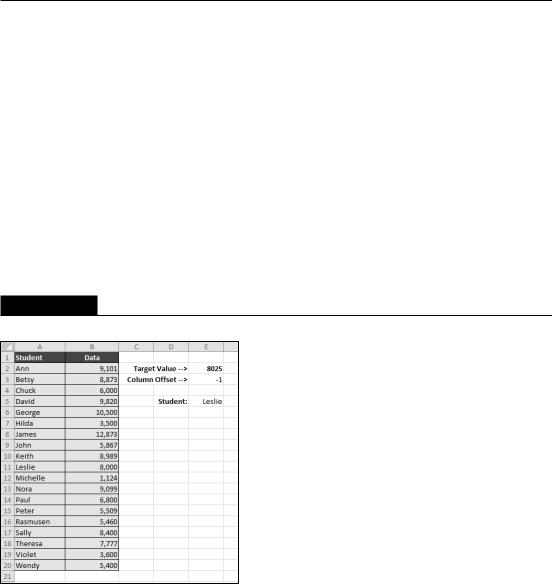
Figure 14.7 illustrates the problem. Suppose that you want to look up the batting average (column B, in a range named Averages) of a player in column C (in a range named Players). The player you want data for appears in a cell named LookupValue. The VLOOKUP function won’t work because the data isn’t arranged correctly. One option is to rearrange your data, but sometimes that’s not possible.

One solution is to use the LOOKUP function, which requires two range arguments. The following formula (in cell F3) returns the batting average from column B of the player name contained in the cell named LookupValue:

=LOOKUP(LookupValue,Players,Averages)

319

Part II: Working with Formulas and Functions

Using the LOOKUP function requires that the lookup range (in this case, the Players range) is in ascending order. In addition to this limitation, the formula suffers from a slight problem: If you enter a nonexistent player (in other words, the LookupValue cell contains a value not found in the Players range), the formula returns an erroneous result.

A better solution uses the INDEX and MATCH functions. The formula that follows works just like the previous one except that it returns #N/A if the player is not found. Another advantage is that the player names need not be sorted.

=INDEX(Averages,MATCH(LookupValue,Players,0))

FIGURE 14.7

The VLOOKUP function can’t look up a value in column B, based on a value in column C.

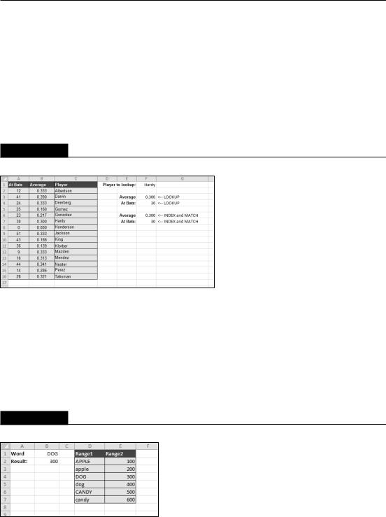
Performing a case-sensitive lookup

The Excel lookup functions (LOOKUP, VLOOKUP, and HLOOKUP) are not case sensitive. For example, if you write a lookup formula to look up the text budget, the formula considers any of the following a match: BUDGET, Budget, or BuDgEt.

Figure 14.8 shows a simple example. Range D2:D7 is named Range1, and range E2:E7 is named Range2. The word to be looked up appears in cell B1 (named Value).

FIGURE 14.8

Using an array formula to perform a case-sensitive lookup.

320

Chapter 14: Creating Formulas That Look Up Values

The array formula that follows is in cell B2. This formula does a case-sensitive lookup in Range1 and returns the corresponding value in Range2.

{=INDEX(Range2,MATCH(TRUE,EXACT(Value,Range1),0))}

The formula looks up the word DOG (uppercase) and returns 300. The following standard LOOKUP formula (which is not case sensitive) returns 400:

=LOOKUP(Value,Range1,Range2)

Note

When entering an array formula, remember to use Ctrl+Shift+Enter. n

Looking up a value from multiple lookup tables

You can, of course, have any number of lookup tables in a worksheet. In some situations, your formula may need to decide which lookup table to use. Figure 14.9 shows an example.

This workbook calculates sales commission and contains two lookup tables: G3:H9 (named CommTable1) and J3:K8 (named CommTable2). The commission rate for a particular sales representative depends on two factors: the sales rep’s years of service (column B) and the amount sold (column C). Column D contains formulas that look up the commission rate from the appropriate table. For example, the formula in cell D2 is

=VLOOKUP(C2,IF(B2<3,CommTable1,CommTable2),2)

FIGURE 14.9

This worksheet demonstrates the use of multiple lookup tables.

The second argument for the VLOOKUP function consists of an IF formula that uses the value in column B to determine which lookup table to use.

The formula in column E simply multiplies the sales amount in column C by the commission rate in column D. The formula in cell E2, for example, is

=C2*D2

321

Part II: Working with Formulas and Functions

Determining letter grades for test scores

A common use of a lookup table is to assign letter grades for test scores. Figure 14.10 shows a worksheet with student test scores. The range E2:F6 (named GradeList) displays a lookup table used to assign a letter grade to a test score.

Column C contains formulas that use the VLOOKUP function and the lookup table to assign a grade based on the score in column B. The formula in cell C2, for example, is

=VLOOKUP(B2,GradeList,2)

When the lookup table is small (as in the example shown earlier in Figure 14.10), you can use a literal array in place of the lookup table. The formula that follows, for example, returns a letter grade without using a lookup table. Rather, the information in the lookup table is hard-coded into an array. See Chapter 17 for more information about arrays.

=VLOOKUP(B2,{0,”F”;40,”D”;70,”C”;80,”B”;90,”A”},2)

Another approach, which uses a more legible formula, is to use the LOOKUP function with two array arguments:

=LOOKUP(B2,{0,40,70,80,90},{“F”,”D”,”C”,”B”,”A”})

FIGURE 14.10

Looking up letter grades for test scores.

Calculating a grade-point average

A student’s grade-point average (GPA) is a numerical measure of the average grade received for classes taken. This discussion assumes a letter grade system, in which each letter grade is assigned a numeric value (A=4, B=3, C=2, D=1, and F=0). The GPA comprises an average of the numeric

322

Chapter 14: Creating Formulas That Look Up Values

grade values weighted by the credit hours of the course. A one-hour course, for example, receives less weight than a three-hour course. The GPA ranges from 0 (all Fs) to 4.00 (all As).

Figure 14.11 shows a worksheet with information for a student. This student took five courses, for a total of 13 credit hours. Range B2:B6 is named CreditHours. The grades for each course appear in column C. (Range C2:C6 is named Grades.) Column D uses a lookup formula to calculate the grade value for each course. The lookup formula in cell D2, for example, follows. This formula uses the lookup table in G2:H6 (named GradeTable).

=VLOOKUP(C2,GradeTable,2,FALSE)

FIGURE 14.11

Using multiple formulas to calculate a GPA.

Formulas in column E calculate the weighted values. The formula in cell E2 is

=D2*B2

Cell B8 computes the GPA by using the following formula:

=SUM(E2:E6)/SUM(B2:B6)

The preceding formulas work fine, but you can streamline the GPA calculation quite a bit. In fact, you can use a single array formula to make this calculation and avoid using the lookup table and the formulas in columns D and E. This array formula does the job:

{=SUM((MATCH(Grades,{“F”,”D”,”C”,”B”,”A”},0)-1)*CreditHours) /SUM(CreditHours)}

Performing a two-way lookup

Figure 14.12 shows a worksheet with a table that displays product sales by month. To retrieve sales for a particular month and product, the user enters a month in cell B1 and a product name in cell B2.

323

Part II: Working with Formulas and Functions

FIGURE 14.12

This table demonstrates a two-way lookup.

To simplify things, the worksheet uses the following named ranges:

The following formula (in cell B4) uses the MATCH function to return the position of the Month within the MonthList range. For example, if the month is January, the formula returns 2 because January is the second item in the MonthList range (the first item is a blank cell, D1).

=MATCH(Month,MonthList,0)

The formula in cell B5 works similarly but uses the ProductList range.

=MATCH(Product,ProductList,0)

The final formula, in cell B6, returns the corresponding sales amount. It uses the INDEX function with the results from cells B4 and B5.

=INDEX(Table,B4,B5)

You can, of course, combine these formulas into a single formula, as shown here:

=INDEX(Table,MATCH(Month,MonthList,0),MATCH(Product,ProductList,0))

324

Chapter 14: Creating Formulas That Look Up Values

Tip

Another way to accomplish a two-way lookup is to provide a name for each row and column of the table. A quick way to do so is to select the table and choose Formulas Defined Names Create from Selection. In the Create Names from Selection dialog box, select the Top Row and Left Column check boxes. After creating the names, you can use a simple formula, such as:

= Sprockets July

This formula, which uses the range intersection operator (a space), returns July sales for Sprockets. See Chapter 10 for details about the range intersection operator. n

Performing a two-column lookup

Some situations may require a lookup based on the values in two columns. Figure 14.13 shows an example.

FIGURE 14.13

This workbook performs a lookup by using information in two columns (D and E).

The lookup table contains automobile makes and models and a corresponding code for each. The worksheet uses named ranges, as shown here:

325

Part II: Working with Formulas and Functions

The following array formula displays the corresponding code for an automobile make and model:

{=INDEX(Code,MATCH(Make&Model,Makes&Models,0))}

This formula works by concatenating the contents of Make and Model and then searching for this text in an array consisting of the concatenated corresponding text in Makes and Models.

Determining the cell address of a value within a range

Most of the time, you want your lookup formula to return a value. You may, however, need to determine the cell address of a particular value within a range. For example, Figure 14.14 shows a worksheet with a range of numbers that occupies a single column (named Data). Cell B1, which contains the value to look up, is named Target.

FIGURE 14.14

The formula in cell B2 returns the address in the Data range for the value in cell B1.

The formula in cell B2, which follows, returns the address of the cell in the Data range that contains the Target value:

=ADDRESS(ROW(Data)+MATCH(Target,Data,0)-1,COLUMN(Data))

If the Data range occupies a single row, use this formula to return the address of the Target value:

=ADDRESS(ROW(Data),COLUMN(Data)+MATCH(Target,Data,0)-1)

If the Data range contains more than one instance of the Target value, the address of the first occurrence is returned. If the Target value isn’t found in the Data range, the formula returns #N/A.

326

Chapter 14: Creating Formulas That Look Up Values

Looking up a value by using the closest match

The VLOOKUP and HLOOKUP functions are useful in the following situations:

•You need to identify an exact match for a target value. Use FALSE as the function’s fourth argument.

•You need to locate an approximate match. If the function’s fourth argument is TRUE or omitted and an exact match is not found, the next largest value less than the lookup value is returned.

But what if you need to look up a value based on the closest match? Neither VLOOKUP nor HLOOKUP can do the job.

Figure 14.15 shows a worksheet with student names in column A and values in column B. Range B2:B20 is named Data. Cell E2, named Target, contains a value to search for in the Data range. Cell E3, named ColOffset, contains a value that represents the column offset from the Data range.

FIGURE 14.15

This workbook demonstrates how to perform a lookup by using the closest match.

The array formula that follows identifies the closest match to the Target value in the Data range and returns the names of the corresponding student in column A (that is, the column with an offset of –1). The formula returns Leslie (with a matching value of 8,000, which is the one closest to the Target value of 8,025).

{=INDIRECT(ADDRESS(ROW(Data)+MATCH(MIN(ABS(Target-Data)), ABS(Target-Data),0)-1,COLUMN(Data)+ColOffset))}

327

Part II: Working with Formulas and Functions

If two values in the Data range are equidistant from the Target value, the formula uses the first one in the list.

The value in ColOffset can be negative (for a column to the left of Data), positive (for a column to the right of Data), or 0 (for the actual closest match value in the Data range).

To understand how this formula works, you need to understand the INDIRECT function. This function’s first argument is a text string in the form of a cell reference (or a reference to a cell that contains a text string). In this example, the text string is created by the ADDRESS function, which accepts a row and column reference and returns a cell address.

328