

- •About the Author
- •About the Technical Editor
- •Credits
- •Is This Book for You?
- •Software Versions
- •Conventions This Book Uses
- •What the Icons Mean
- •How This Book Is Organized
- •How to Use This Book
- •What’s on the Companion CD
- •What Is Excel Good For?
- •What’s New in Excel 2010?
- •Moving around a Worksheet
- •Introducing the Ribbon
- •Using Shortcut Menus
- •Customizing Your Quick Access Toolbar
- •Working with Dialog Boxes
- •Using the Task Pane
- •Creating Your First Excel Worksheet
- •Entering Text and Values into Your Worksheets
- •Entering Dates and Times into Your Worksheets
- •Modifying Cell Contents
- •Applying Number Formatting
- •Controlling the Worksheet View
- •Working with Rows and Columns
- •Understanding Cells and Ranges
- •Copying or Moving Ranges
- •Using Names to Work with Ranges
- •Adding Comments to Cells
- •What Is a Table?
- •Creating a Table
- •Changing the Look of a Table
- •Working with Tables
- •Getting to Know the Formatting Tools
- •Changing Text Alignment
- •Using Colors and Shading
- •Adding Borders and Lines
- •Adding a Background Image to a Worksheet
- •Using Named Styles for Easier Formatting
- •Understanding Document Themes
- •Creating a New Workbook
- •Opening an Existing Workbook
- •Saving a Workbook
- •Using AutoRecover
- •Specifying a Password
- •Organizing Your Files
- •Other Workbook Info Options
- •Closing Workbooks
- •Safeguarding Your Work
- •Excel File Compatibility
- •Exploring Excel Templates
- •Understanding Custom Excel Templates
- •Printing with One Click
- •Changing Your Page View
- •Adjusting Common Page Setup Settings
- •Adding a Header or Footer to Your Reports
- •Copying Page Setup Settings across Sheets
- •Preventing Certain Cells from Being Printed
- •Preventing Objects from Being Printed
- •Creating Custom Views of Your Worksheet
- •Understanding Formula Basics
- •Entering Formulas into Your Worksheets
- •Editing Formulas
- •Using Cell References in Formulas
- •Using Formulas in Tables
- •Correcting Common Formula Errors
- •Using Advanced Naming Techniques
- •Tips for Working with Formulas
- •A Few Words about Text
- •Text Functions
- •Advanced Text Formulas
- •Date-Related Worksheet Functions
- •Time-Related Functions
- •Basic Counting Formulas
- •Advanced Counting Formulas
- •Summing Formulas
- •Conditional Sums Using a Single Criterion
- •Conditional Sums Using Multiple Criteria
- •Introducing Lookup Formulas
- •Functions Relevant to Lookups
- •Basic Lookup Formulas
- •Specialized Lookup Formulas
- •The Time Value of Money
- •Loan Calculations
- •Investment Calculations
- •Depreciation Calculations
- •Understanding Array Formulas
- •Understanding the Dimensions of an Array
- •Naming Array Constants
- •Working with Array Formulas
- •Using Multicell Array Formulas
- •Using Single-Cell Array Formulas
- •Working with Multicell Array Formulas
- •What Is a Chart?
- •Understanding How Excel Handles Charts
- •Creating a Chart
- •Working with Charts
- •Understanding Chart Types
- •Learning More
- •Selecting Chart Elements
- •User Interface Choices for Modifying Chart Elements
- •Modifying the Chart Area
- •Modifying the Plot Area
- •Working with Chart Titles
- •Working with a Legend
- •Working with Gridlines
- •Modifying the Axes
- •Working with Data Series
- •Creating Chart Templates
- •Learning Some Chart-Making Tricks
- •About Conditional Formatting
- •Specifying Conditional Formatting
- •Conditional Formats That Use Graphics
- •Creating Formula-Based Rules
- •Working with Conditional Formats
- •Sparkline Types
- •Creating Sparklines
- •Customizing Sparklines
- •Specifying a Date Axis
- •Auto-Updating Sparklines
- •Displaying a Sparkline for a Dynamic Range
- •Using Shapes
- •Using SmartArt
- •Using WordArt
- •Working with Other Graphic Types
- •Using the Equation Editor
- •Customizing the Ribbon
- •About Number Formatting
- •Creating a Custom Number Format
- •Custom Number Format Examples
- •About Data Validation
- •Specifying Validation Criteria
- •Types of Validation Criteria You Can Apply
- •Creating a Drop-Down List
- •Using Formulas for Data Validation Rules
- •Understanding Cell References
- •Data Validation Formula Examples
- •Introducing Worksheet Outlines
- •Creating an Outline
- •Working with Outlines
- •Linking Workbooks
- •Creating External Reference Formulas
- •Working with External Reference Formulas
- •Consolidating Worksheets
- •Understanding the Different Web Formats
- •Opening an HTML File
- •Working with Hyperlinks
- •Using Web Queries
- •Other Internet-Related Features
- •Copying and Pasting
- •Copying from Excel to Word
- •Embedding Objects in a Worksheet
- •Using Excel on a Network
- •Understanding File Reservations
- •Sharing Workbooks
- •Tracking Workbook Changes
- •Types of Protection
- •Protecting a Worksheet
- •Protecting a Workbook
- •VB Project Protection
- •Related Topics
- •Using Excel Auditing Tools
- •Searching and Replacing
- •Spell Checking Your Worksheets
- •Using AutoCorrect
- •Understanding External Database Files
- •Importing Access Tables
- •Retrieving Data with Query: An Example
- •Working with Data Returned by Query
- •Using Query without the Wizard
- •Learning More about Query
- •About Pivot Tables
- •Creating a Pivot Table
- •More Pivot Table Examples
- •Learning More
- •Working with Non-Numeric Data
- •Grouping Pivot Table Items
- •Creating a Frequency Distribution
- •Filtering Pivot Tables with Slicers
- •Referencing Cells within a Pivot Table
- •Creating Pivot Charts
- •Another Pivot Table Example
- •Producing a Report with a Pivot Table
- •A What-If Example
- •Types of What-If Analyses
- •Manual What-If Analysis
- •Creating Data Tables
- •Using Scenario Manager
- •What-If Analysis, in Reverse
- •Single-Cell Goal Seeking
- •Introducing Solver
- •Solver Examples
- •Installing the Analysis ToolPak Add-in
- •Using the Analysis Tools
- •Introducing the Analysis ToolPak Tools
- •Introducing VBA Macros
- •Displaying the Developer Tab
- •About Macro Security
- •Saving Workbooks That Contain Macros
- •Two Types of VBA Macros
- •Creating VBA Macros
- •Learning More
- •Overview of VBA Functions
- •An Introductory Example
- •About Function Procedures
- •Executing Function Procedures
- •Function Procedure Arguments
- •Debugging Custom Functions
- •Inserting Custom Functions
- •Learning More
- •Why Create UserForms?
- •UserForm Alternatives
- •Creating UserForms: An Overview
- •A UserForm Example
- •Another UserForm Example
- •More on Creating UserForms
- •Learning More
- •Why Use Controls on a Worksheet?
- •Using Controls
- •Reviewing the Available ActiveX Controls
- •Understanding Events
- •Entering Event-Handler VBA Code
- •Using Workbook-Level Events
- •Working with Worksheet Events
- •Using Non-Object Events
- •Working with Ranges
- •Working with Workbooks
- •Working with Charts
- •VBA Speed Tips
- •What Is an Add-In?
- •Working with Add-Ins
- •Why Create Add-Ins?
- •Creating Add-Ins
- •An Add-In Example
- •System Requirements
- •Using the CD
- •What’s on the CD
- •Troubleshooting
- •The Excel Help System
- •Microsoft Technical Support
- •Internet Newsgroups
- •Internet Web sites
- •End-User License Agreement

Part V: Analyzing Data with Excel
FIGURE 34.19
This pivot table uses three Report Filters.
Learning More
The examples in this chapter should give you an appreciation for the power and flexibility of Excel pivot tables. The next chapter digs a bit deeper and covers some advanced features — with lots of examples.
714
CHAPTER
Analyzing Data with
Pivot Tables
The previous chapter introduces pivot tables. There, I present several examples to demonstrate the types of pivot table summaries that you can generate from a set of data.
This chapter continues the discussion and explores the details of creating effective pivot tables. Creating a basic pivot table is very easy, and the examples in this chapter demonstrate additional pivot table features that you may find helpful. I urge you to try these techniques with your own data. If you don’t have suitable data, use the files on the companion CD-ROM.
Working with Non-Numeric Data
Most pivot tables are created from numeric data, but pivot tables are also useful with some types of non-numeric data. Because you can’t sum nonnumbers, this technique involves counting.
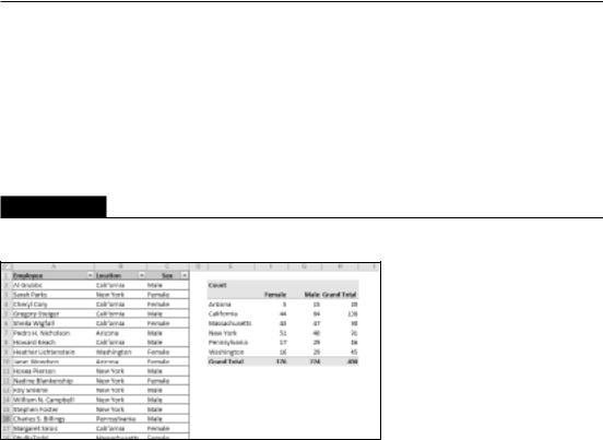
Figure 35.1 shows a table and a pivot table generated from the table. The table is a list of 400 employees, along with their location and gender. As you can see, the table has no numeric values, but you can create a useful pivot table that counts the items rather than sums them. The pivot table crosstabulates the Location field by the Sex field for the 400 employees and shows the count for each combination of location and gender.
On the CD
A workbook that demonstrates the pivot table created from non-numeric data is available on the companion CD-ROM. The file is named employee list. xlsx.
IN THIS CHAPTER
How to create a pivot table from non-numeric data
How to group items in a pivot table
How to create a calculated field or a calculated item in a pivot table
How to create an attractive report using a pivot table
715
Part V: Analyzing Data with Excel
Here are the settings I used for this pivot table:
•The Sex field is used for the Column Labels.
•The Location field is used for the Row Labels.
•Location is used for the Values and is summarized by Count.
•The pivot table has the field headers turned off (by choosing PivotTable Tools OptionsShow Show Field headers).
FIGURE 35.1
This table doesn’t have any numeric fields, but you can use it to generate a pivot table, shown next to the table.
Note
The Employee field is not used. This example uses the Location field for the Values section, but you can actually use any of the three fields because the pivot table is displaying a count. n
Figure 35.2 shows the pivot table after making some additional changes:
•I added a second instance of the Location field to the Values section. To display percentages, I right-clicked a value in that column, and chose Show Values As Percent of Column Total.
•I changed the field names in the pivot table to Count and Pct.
•I selected a Pivot Table Style that makes it easier to distinguish the columns.
716

Chapter 35: Analyzing Data with Pivot Tables
FIGURE 35.2
The pivot table, after making a few changes.
Grouping Pivot Table Items
One of the most useful features of a pivot table is the ability to combine items into groups. You can group items that appear as Row Labels or Column Labels. Excel offers two ways to group items:
•Manually: After creating the pivot table, select the items to be grouped and then choose PivotTable Tools Options Group Group Selection. Or, you can right-click and choose Group from the shortcut menu.
•Automatically: If the items are numeric (or dates), use the Grouping dialog box to specify how you would like to group the items. Select any item in the Row Labels or Column Labels and then choose PivotTable Tools Options Group Group Selection. Or, you can right-click and choose Group from the shortcut menu. In either case, Excel displays its Grouping dialog box.
A manual grouping example
Figure 35.3 shows the pivot table example from the previous sections, with two groups created from the Row Labels. To create the first group, I held the Ctrl key while I selected Arizona, California, and Washington. Then I right-clicked and chose Group from the shortcut menu. Excel created a second group automatically. Then I replaced the default group names (Group 1 and Group 2) with more meaningful names (Western Region and Eastern Region).
You can create any number of groups, and even create groups of groups.
Excel provides a number of options for displaying a pivot table, and you may want to experiment with these options when you use groups. These commands are on the PivotTable Tools Design tab of the Ribbon. There are no rules for choosing a particular option. The key is to try a few and see which makes your pivot table look the best. In addition, try various PivotTable Styles, with options for banded rows or banded columns. Often, the style that you choose can greatly enhance readability.
717

Part V: Analyzing Data with Excel
FIGURE 35.3
A pivot table with two groups.
Figure 35.4 shows pivot tables using various options for displaying subtotals, grand totals, and styles.
FIGURE 35.4
Pivot tables with options for subtotals and grand totals.
718

Chapter 35: Analyzing Data with Pivot Tables
Automatic grouping examples
When a field contains numbers, dates, or times, Excel can create groups automatically. The two examples in this section demonstrate automatic grouping.
Grouping by date
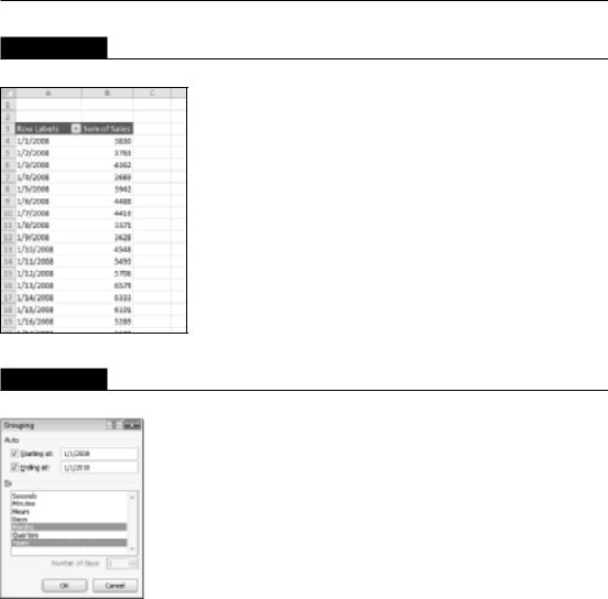
Figure 35.5 shows a portion of a simple table with two fields: Date and Sales. This table has 730 rows and covers the dates between January 1, 2008 and December 31, 2009. The goal is to summarize the sales information by month.
FIGURE 35.5
You can use a pivot table to summarize the sales data by month.
On the CD
A workbook demonstrating how to group pivot table items by date is available on the companion CD-ROM. The file is named sales by date.xlsx.
Figure 35.6 shows part of a pivot table created from the data. The Date field is in the Row Labels section, and the Sales field is in the Values section. Not surprisingly, the pivot table looks exactly like the input data because the dates have not been grouped.
To group the items by month, select any date and choose PivotTable Tools Options Group Group Field (or, right-click and choose Group from the shortcut menu). You see the Grouping dialog box, shown in Figure 35.7. Excel supplies values for the Starting At and Ending At fields. The values cover the entire range of data, and you can change them if you like.
719
Part V: Analyzing Data with Excel
FIGURE 35.6
The pivot table, before grouping by month.
FIGURE 35.7
Use the Grouping dialog box to group pivot table items by dates.
In the By list box, select Months and Years and verify that the starting and ending dates are correct for your data. Click OK. The Date items in the pivot table are grouped by years and by months, as shown in Figure 35.8.
Note
If you select only Months in the By list box in the Grouping dialog box, months in different years combine together. For example, the January item would display sales for both 2008 and 2009. n
720

Chapter 35: Analyzing Data with Pivot Tables
FIGURE 35.8
The pivot table, after grouping by month and year.
Figure 35.9 shows another view of the data, grouped by quarter and by year.
FIGURE 35.9
This pivot table shows sales by quarter and by year.
721