Chapter 10: Introducing Formulas and Functions

•As you become familiar with the functions, you can bypass the Insert Function dialog box and type the function name directly. Excel prompts you with argument names as you enter the function.

Editing Formulas

After you enter a formula, you can (of course) edit that formula. You may need to edit a formula if you make some changes to your worksheet and then have to adjust the formula to accommodate the changes. Or the formula may return an error value, in which case you have to edit the formula to correct the error.

The following are some of the ways to get into cell edit mode:

•Double-click the cell, which enables you to edit the cell contents directly in the cell.

•Press F2, which enables you to edit the cell contents directly in the cell.

•Select the cell that you want to edit, and then click in the Formula bar. This enables you to edit the cell contents in the Formula bar.

•If the cell contains a formula that returns an error, Excel will display a small triangle in the upper-left corner of the cell. Activate the cell, and you’ll see a Smart Tag. Click the Smart Tag, and you can choose one of the options for correcting the error. (The options will vary according to the type of error in the cell.)

Tip

You can control whether Excel displays these formula-error–checking Smart Tags in the Formulas section of the Excel Options dialog box. To display this dialog box, choose File Options. If you remove the check mark from Enable Background Error Checking, Excel no longer displays these Smart Tags. n

While you’re editing a formula, you can select multiple characters either by dragging the mouse cursor over them or by pressing Shift while you use the navigation keys.

Tip

If you have a formula that you can’t seem to edit correctly, you can convert the formula to text and tackle it again later. To convert a formula to text, just remove the initial equal sign (=). When you’re ready to try again, type the initial equal sign to convert the cell contents back to a formula. n

Using Cell References in Formulas

Most formulas you create include references to cells or ranges. These references enable your formulas to work dynamically with the data contained in those cells or ranges. For example, if your formula refers to cell A1 and you change the value contained in A1, the formula result changes to

209

Part II: Working with Formulas and Functions

reflect the new value. If you didn’t use references in your formulas, you would need to edit the formulas themselves in order to change the values used in the formulas.

Using relative, absolute, and mixed references

When you use a cell (or range) reference in a formula, you can use three types of references:

•Relative: The row and column references can change when you copy the formula to another cell because the references are actually offsets from the current row and column. By default, Excel creates relative cell references in formulas.

•Absolute: The row and column references do not change when you copy the formula because the reference is to an actual cell address. An absolute reference uses two dollar signs in its address: one for the column letter and one for the row number (for example, $A$5).

•Mixed: Either the row or column reference is relative, and the other is absolute. Only one of the address parts is absolute (for example, $A4 or A$4).

The type of cell reference is important only if you plan to copy the formula to other cells. The following examples illustrate this point.

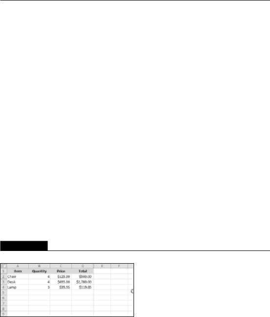
Figure 10.7 shows a simple worksheet. The formula in cell D2, which multiplies the quantity by the price, is

=B2*C2

This formula uses relative cell references. Therefore, when the formula is copied to the cells below it, the references adjust in a relative manner. For example, the formula in cell D3 is

=B3*C3

FIGURE 10.7

Copying a formula that contains relative references.

But what if the cell references in D2 contained absolute references, like this?

=$B$2*$C$2

210

Chapter 10: Introducing Formulas and Functions

In this case, copying the formula to the cells below would produce incorrect results. The formula in cell D3 would be exactly the same as the formula in cell D2.

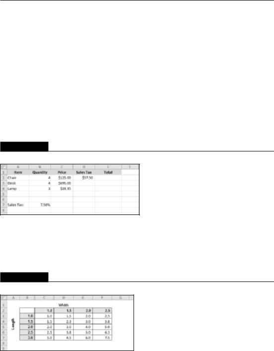
Now I’ll extend the example to calculate sales tax, which is stored in cell B7 (see Figure 10.8). In this situation, the formula in cell D2 is

=(B2*C2)*$B$7

The quantity is multiplied by the price, and the result is multiplied by the sales-tax rate stored in cell B7. Notice that the reference to B7 is an absolute reference. When the formula in D2 is copied to the cells below it, cell D3 will contain this formula:

=(B3*C3)*$B$7

Here, the references to cells B2 and C2 were adjusted, but the reference to cell B7 was not — which is exactly what I want because the cell that contains the sales tax never changes.

FIGURE 10.8

Formula references to the sales tax cell should be absolute.

Figure 10.9 demonstrates the use of mixed references. The formulas in the C3:F7 range calculate the area for various lengths and widths. The formula in cell C3 is

=$B3*C$2

FIGURE 10.9

Using mixed cell references.

211

Part II: Working with Formulas and Functions

Notice that both cell references are mixed. The reference to cell B3 uses an absolute reference for the column ($B), and the reference to cell C2 uses an absolute reference for the row ($2). As a result, this formula can be copied down and across, and the calculations will be correct. For example, the formula in cell F7 is

=$B7*F$2

If C3 used either absolute or relative references, copying the formula would produce incorrect results.

On the CD

The workbook that demonstrates the various types of references is available on the companion CD-ROM. The file is named cell references.xlsx.

Note

When you cut and paste a formula (move it to another location), the cell references in the formula aren’t adjusted. Again, this is usually what you want to happen. When you move a formula, you generally want it to continue to refer to the original cells. n

Changing the types of your references

You can enter nonrelative references (that is, absolute or mixed) manually by inserting dollar signs in the appropriate positions of the cell address. Or you can use a handy shortcut: the F4 key. When you’ve entered a cell reference (by typing it or by pointing), you can press F4 repeatedly to have Excel cycle through all four reference types.

For example, if you enter =A1 to start a formula, pressing F4 converts the cell reference to =$A$1. Pressing F4 again converts it to =A$1. Pressing it again displays =$A1. Pressing it one more time returns to the original =A1. Keep pressing F4 until Excel displays the type of reference that you want.

Note

When you name a cell or range, Excel (by default) uses an absolute reference for the name. For example, if you give the name SalesForecast to B1:B12, the Refers To box in the New Name dialog box lists the reference as $B$1:$B$12. This is almost always what you want. If you copy a cell that has a named reference in its formula, the copied formula contains a reference to the original name. n

Referencing cells outside the worksheet

Formulas can also refer to cells in other worksheets — and the worksheets don’t even have to be in the same workbook. Excel uses a special type of notation to handle these types of references.

212

Chapter 10: Introducing Formulas and Functions

Referencing cells in other worksheets

To use a reference to a cell in another worksheet in the same workbook, use this format:

SheetName!CellAddress

In other words, precede the cell address with the worksheet name, followed by an exclamation point. Here’s an example of a formula that uses a cell on the Sheet2 worksheet:

=A1*Sheet2!A1

This formula multiplies the value in cell A1 on the current worksheet by the value in cell A1 on

Sheet2.

Tip

If the worksheet name in the reference includes one or more spaces, you must enclose it in single quotation marks. (Excel does that automatically if you use the point-and-click method.) For example, here’s a formula that refers to a cell on a sheet named All Depts:

=A1*’All Depts’! A1

Referencing cells in other workbooks

To refer to a cell in a different workbook, use this format:

=[WorkbookName]SheetName!CellAddress

In this case, the workbook name (in square brackets), the worksheet name, and an exclamation point precede the cell address. The following is an example of a formula that uses a cell reference in the Sheet1 worksheet in a workbook named Budget:

=[Budget.xlsx]Sheet1!A1

If the workbook name in the reference includes one or more spaces, you must enclose it (and the sheet name) in single quotation marks. For example, here’s a formula that refers to a cell on

Sheet1 in a workbook named Budget For 2011:

=A1*’[Budget For 2011.xlsx]Sheet1’!A1

When a formula refers to cells in a different workbook, the other workbook doesn’t have to be open. If the workbook is closed, however, you must add the complete path to the reference so that Excel can find it. Here’s an example:

=A1*’C:\My Documents\[Budget For 2011.xlsx]Sheet1’!A1

A linked file can also reside on another system that’s accessible on your corporate network. The following formula refers to a cell in a workbook in the files directory of a computer named

DataServer.

=’\\DataServer\files\[budget.xlsx]Sheet1’!$D$7

213