Part II: Working with Formulas and Functions

Determining a date’s quarter

For financial reports, you may find it useful to present information in terms of quarters. The following formula returns an integer between 1 and 4 that corresponds to the calendar quarter for the date in cell A1:

=ROUNDUP(MONTH(A1)/3,0)

This formula divides the month number by 3 and then rounds up the result.

Time-Related Functions

Excel also includes a number of functions that enable you to work with time values in your formulas. This section contains examples that demonstrate the use of these functions.

Table 12.5 summarizes the time-related functions available in Excel. These functions work with date serial numbers. When you use the Insert Function dialog box, these functions appear in the Date & Time function category.

TABLE 12.5

Displaying the current time

This formula displays the current time as a time serial number (or as a serial number without an associated date):

=NOW()-TODAY()

You need to format the cell with a time format to view the result as a recognizable time. The quickest way is to choose Home Number Format Number and select Time from the drop-down list.

272

Chapter 12: Working with Dates and Times

Note

This formula is updated only when the worksheet is calculated. n

Tip

To enter a time stamp (that doesn’t change) into a cell, press Ctrl+Shift+: (colon). n

Displaying any time

One way to enter a time value into a cell is to just type it, making sure that you include at least one colon (:). You can also create a time by using the TIME function. For example, the following formula returns a time comprising of the hour in cell A1, the minute in cell B1, and the second in cell C1:

=TIME(A1,B1,C1)

Like the DATE function, the TIME function accepts invalid arguments and adjusts the result accordingly. For example, the following formula uses 80 as the minute argument and returns 10:20:15 AM. The 80 minutes are simply added to the hour, with 20 minutes remaining.

=TIME(9,80,15)

Caution

If you enter a value greater than 24 as the first argument for the TIME function, the result may not be what you expect. Logically, a formula such as the one that follows should produce a date/time serial number of 1.041667 (that is, one day and one hour).

=TIME(25,0,0)

In fact, this formula is equivalent to the following:

=TIME(1,0,0)

You can also use the DATE function along with the TIME function in a single cell. The formula that follows generates a date and time with a serial number of 39420.7708333333 — which represents 6:30 PM on December 4, 2010:

=DATE(2010,12,4)+TIME(18,30,0)

The TIMEVALUE function converts a text string that looks like a time into a time serial number. This formula returns 0.2395833333, the time serial number for 5:45 AM:

=TIMEVALUE(“5:45 am”)

To view the result of this formula as a time, you need to apply number formatting to the cell. The TIMEVALUE function doesn’t recognize all common time formats. For example, the following formula returns an error because Excel doesn’t like the periods in “a.m.”

=TIMEVALUE(“5:45 a.m.”)

273

Part II: Working with Formulas and Functions

Calculating the difference between two times

Because times are represented as serial numbers, you can subtract the earlier time from the later time to get the difference. For example, if cell A2 contains 5:30:00 and cell B2 contains 14:00:00, the following formula returns 08:30:00 (a difference of 8 hours and 30 minutes):

=B2-A2

If the subtraction results in a negative value, however, it becomes an invalid time; Excel displays a series of hash marks (#######) because a time without a date has a date serial number of 0. A negative time results in a negative serial number, which cannot be displayed — although you can still use the calculated value in other formulas.

If the direction of the time difference doesn’t matter, you can use the ABS function to return the absolute value of the difference:

=ABS(B2-A2)

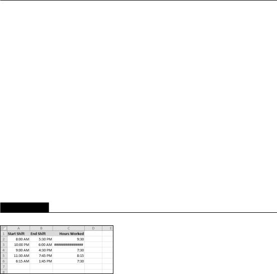
This “negative time” problem often occurs when calculating an elapsed time — for example, calculating the number of hours worked given a start time and an end time. This presents no problem if the two times fall in the same day. But if the work shift spans midnight, the result is an invalid negative time. For example, you may start work at 10:00 p.m. and end work at 6:00 a.m. the next day. Figure 12.7 shows a worksheet that calculates the hours worked. As you can see, the shift that spans midnight presents a problem (cell C3).

FIGURE 12.7

Calculating the number of hours worked returns an error if the shift spans midnight.

Using the ABS function (to calculate the absolute value) isn’t an option in this case because it returns the wrong result (16 hours). The following formula, however, does work:

=IF(B2<A2,B2+1,B2)-A2

274

Chapter 12: Working with Dates and Times

Tip

Negative times are permitted if the workbook uses the 1904 date system. To switch to the 1904 date system, use the Advanced section of the Excel Options dialog box. Select the Use 1904 Date System option. But beware! When changing the workbook’s date system, if the workbook uses dates, the dates will be off by four years For more information about the 1904 date system, see the sidebar “Choose Your Date System: 1900 or 1904,” earlier in this chapter. n

Summing times that exceed 24 hours

Many people are surprised to discover that when you sum a series of times that exceed 24 hours, Excel doesn’t display the correct total. Figure 12.8 shows an example. The range B2:B8 contains times that represent the hours and minutes worked each day. The formula in cell B9 is

=SUM(B2:B8)

As you can see, the formula returns a seemingly incorrect total (17 hours, 45 minutes). The total should read 41 hours, 45 minutes. The problem is that the formula is displaying the total as a date/ time serial number of 1.7395833, but the cell formatting is not displaying the date part of the date/ time. The answer is incorrect because cell B9 has the wrong number format.

FIGURE 12.8

Incorrect cell formatting makes the total appear incorrectly.

To view a time that exceeds 24 hours, you need to apply a custom number format for the cell so that square brackets surround the hour part of the format string. Applying the number format here to cell B9 displays the sum correctly:

[h]:mm

Cross-Reference

For more information about custom number formats, see Chapter 24. n

275

Part II: Working with Formulas and Functions

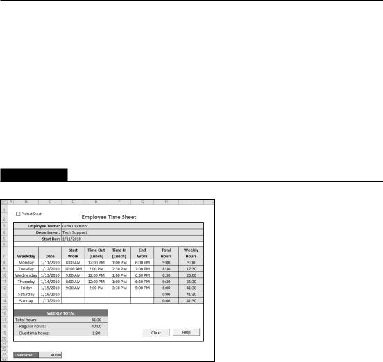
Figure 12.9 shows another example of a worksheet that manipulates times. This worksheet keeps track of hours worked during a week (regular hours and overtime hours).

On the CD

This workbook is available on the companion CD-ROM. The filename is time sheet.xlsm. The workbook contains a few macros to make it easier to use. n

The week’s starting date appears in cell D5, and the formulas in column B fill in the dates for the days of the week. Times appear in the range D8:G14, and formulas in column H calculate the number of hours worked each day. For example, the formula in cell H8 is

=IF(E8<D8,E8+1-D8,E8-D8)+IF(G8<F8,G8+1-G8,G8-F8)

FIGURE 12.9

An employee timesheet workbook.

The first part of this formula subtracts the time in column D from the time in column E to get the total hours worked before lunch. The second part subtracts the time in column F from the time in column G to get the total hours worked after lunch. I use IF functions to accommodate graveyard shift cases that span midnight — for example, an employee may start work at 10:00 PM and begin lunch at 2:00 AM. Without the IF function, the formula returns a negative result.

The following formula in cell H17 calculates the weekly total by summing the daily totals in column H:

=SUM(H8:H14)

276

Chapter 12: Working with Dates and Times

This worksheet assumes that hours in excess of 40 hours in a week are considered overtime hours. The worksheet contains a cell named Overtime, in cell C23. This cell contains a formula that returns 40:00. If your standard workweek consists of something other than 40 hours, you can change this cell.

The following formula (in cell H18) calculates regular (nonovertime) hours. This formula returns the smaller of two values: the total hours or the overtime hours.

=MIN(E17,Overtime)

The final formula, in cell H19, simply subtracts the regular hours from the total hours to yield the overtime hours.

=E17-E18

The times in H17:H19 may display time values that exceed 24 hours, so these cells use a custom number format:

[h]:mm

Converting from military time

Military time is expressed as a four-digit number from 0000 to 2359. For example, 1:00 a.m. is expressed as 0100 hours, and 3:30 p.m. is expressed as 1530 hours. The following formula converts such a number (assumed to be in cell A1) to a standard time:

=TIMEVALUE(LEFT(A1,2)&”:”&RIGHT(A1,2))

The formula returns an incorrect result if the contents of cell A1 do not contain four digits. The following formula corrects the problem, and it returns a valid time for any military time value from

0 to 2359:

=TIMEVALUE(LEFT(TEXT(A1,”0000”),2)&”:”&RIGHT(A1,2))

Following is a simpler formula that uses the TEXT function to return a formatted string, and then it uses the TIMEVALUE function to express the result in terms of a time.

=TIMEVALUE(TEXT(A1,”00\:00”))

Converting decimal hours, minutes, or seconds to a time

To convert decimal hours to a time, divide the decimal hours by 24. For example, if cell A1 contains 9.25 (representing hours), this formula returns 09:15:00 (nine hours, 15 minutes):

=A1/24

277

Part II: Working with Formulas and Functions

To convert decimal minutes to a time, divide the decimal hours by 1,440 (the number of minutes in a day). For example, if cell A1 contains 500 (representing minutes), the following formula returns 08:20:00 (eight hours, 20 minutes):

=A1/1440

To convert decimal seconds to a time, divide the decimal hours by 86,400 (the number of seconds in a day). For example, if cell A1 contains 65,000 (representing seconds), the following formula returns 18:03:20 (18 hours, three minutes, and 20 seconds):

=A1/86400

Adding hours, minutes, or seconds to a time

You can use the TIME function to add any number of hours, minutes, or seconds to a time. For example, assume that cell A1 contains a time. The following formula adds 2 hours and 30 minutes to that time and displays the result:

=A1+TIME(2,30,0)

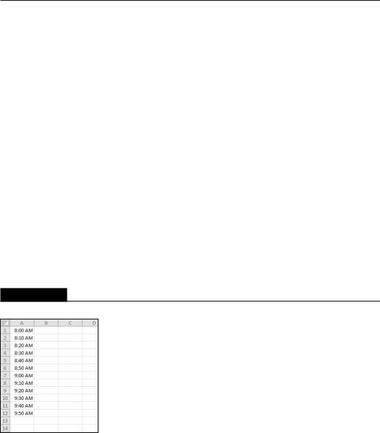
You can use the TIME function to fill a range of cells with incremental times. Figure 12.10 shows a worksheet with a series of times in 10-minute increments. Cell A1 contains a time that was entered directly. Cell A2 contains the following formula, which copied down the column:

=A1+TIME(0,10,0)

FIGURE 12.10

Using a formula to create a series of incremental times.

278

Chapter 12: Working with Dates and Times

Rounding time values

You may need to create a formula that rounds a time to a particular value. For example, you may need to enter your company’s time records rounded to the nearest 15 minutes. This section presents examples of various ways to round a time value.

The following formula rounds the time in cell A1 to the nearest minute:

=ROUND(A1*1440,0)/1440

The formula works by multiplying the time by 1440 (to get total minutes). This value is passed to the ROUND function, and the result is divided by 1440. For example, if cell A1 contains 11:52:34, the formula returns 11:53:00.

The following formula resembles this example, except that it rounds the time in cell A1 to the nearest hour:

=ROUND(A1*24,0)/24

If cell A1 contains 5:21:31, the formula returns 5:00:00.

The following formula rounds the time in cell A1 to the nearest 15 minutes (a quarter of an hour):

=ROUND(A1*24/0.25,0)*(0.25/24)

In this formula, 0.25 represents the fractional hour. To round a time to the nearest 30 minutes, change 0.25 to 0.5, as in the following formula:

=ROUND(A1*24/0.5,0)*(0.5/24)

Working with non–time-of-day values

Sometimes, you may want to work with time values that don’t represent an actual time of day. For example, you may want to create a list of the finish times for a race or record the amount of time you spend in meetings each day. Such times don’t represent a time of day. Rather, a value represents the time for an event (in hours, minutes, and seconds). The time to complete a test, for example, may be 35 minutes and 45 seconds. You can enter that value into a cell as:

00:35:45

Excel interprets such an entry as 12:35:45 a.m., which works fine. (Just make sure that you format the cell so that it appears as you like.) When you enter such times that do not have an hour component, you must include at least one zero for the hour. If you omit a leading zero for a missing hour, Excel interprets your entry as 35 hours and 45 minutes.

279

Part II: Working with Formulas and Functions

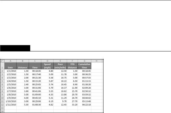
Figure 12.11 shows an example of a worksheet set up to keep track of a person’s jogging activity. Column A contains simple dates. Column B contains the distance in miles. Column C contains the time it took to run the distance. Column D contains formulas to calculate the speed in miles per hour. For example, the formula in cell D2 is

=B2/(C2*24)

FIGURE 12.11

This worksheet uses times not associated with a time of day.

Column E contains formulas to calculate the pace, in minutes per mile. For example, the formula in cell E2 is

=(C2*60*24)/B2

Columns F and G contain formulas that calculate the year-to-date distance (using column B) and the cumulative time (using column C). The cells in column G are formatted using the following number format (which permits time displays that exceed 24 hours):

[hh]:mm:ss

On the CD

You can also access the workbook shown in Figure 12.11 on the companion CD-ROM. The file is named jogging log.xlsx.

280

CHAPTER

Creating Formulas

That Count and Sum

281

Part II: Working with Formulas and Functions

Note

If your data is in the form of a table, you can use autofiltering to accomplish many counting and summing operations. Just set the autofilter criteria, and the table displays only the rows that match your criteria (the nonqualifying rows in the table are hidden). Then you can select formulas to display counts or sums in the table’s total row. See Chapter 5 for more information on using tables. n

TABLE 13.1

* These functions were introduced in Excel 2007.

282