CHAPTER

Introducing Formulas

and Functions

195

Part II: Working with Formulas and Functions

Note

When you’re working with a table, a feature introduced in Excel 2007 enables you to create formulas that use column names from the table — which can make your formulas much easier to read. I discuss table formulas later in this chapter. (See “Using Formulas In Tables.”) n

After you enter a formula, the cell displays the calculated result of the formula. The formula itself appears in the Formula bar when you select the cell, however.

Here are a few examples of formulas:

Tip

Formulas always begin with an equal sign so that Excel can distinguish them from text. n

Using operators in formulas

Excel lets you use a variety of operators in your formulas. Operators are symbols that indicate what mathematical operation you want the formula to perform. Table 10.1 lists the operators that Excel recognizes. In addition to these, Excel has many built-in functions that enable you to perform additional calculations.

TABLE 10.1

196

You can, of course, use as many operators as you need to perform the desired calculation.

Here are some examples of formulas that use various operators.

Understanding operator precedence in formulas

When Excel calculates the value of a formula, it uses certain rules to determine the order in which the various parts of the formula are calculated. You need to understand these rules if you want your formulas to produce the desired results.

Table 10.2 lists the Excel operator precedence. This table shows that exponentiation has the highest precedence (performed first) and logical comparisons have the lowest precedence (performed last).

197

Part II: Working with Formulas and Functions

TABLE 10.2

Operator Precedence in Excel Formulas

You can use parentheses to override the Excel’s built-in order of precedence. Expressions within parentheses are always evaluated first. For example, the following formula uses parentheses to control the order in which the calculations occur. In this case, cell B3 is subtracted from cell B2, and the result is multiplied by cell B4:

=(B2-B3)*B4

If you enter the formula without the parentheses, Excel computes a different answer. Because multiplication has a higher precedence, cell B3 is multiplied by cell B4. Then this result is subtracted from cell B2, which isn’t what was intended.

The formula without parentheses looks like this:

=B2-B3*B4

It’s a good idea to use parentheses even when they aren’t strictly necessary. Doing so helps to clarify what the formula is intended to do. For example, the following formula makes it perfectly clear that B3 should be multiplied by B4, and the result subtracted from cell B2. Without the parentheses, you would need to remember Excel’s order of precedence.

=B2-(B3*B4)

You can also nest parentheses within formulas — that is, put them inside other parentheses. If you do so, Excel evaluates the most deeply nested expressions first — and then works its way out. Here’s an example of a formula that uses nested parentheses:

=((B2*C2)+(B3*C3)+(B4*C4))*B6

198

Chapter 10: Introducing Formulas and Functions

This formula has four sets of parentheses — three sets are nested inside the fourth set. Excel evaluates each nested set of parentheses and then sums the three results. This result is then multiplied by the value in cell B6.

Although the preceding formula uses four sets of parentheses, only the outer set is really necessary. If you understand operator precedence, it should be clear that you can rewrite this formula as:

=(B2*C2+B3*C3+B4*C4)*B6

But most would agree that using the extra parentheses makes the calculation much clearer.

Every left parenthesis, of course, must have a matching right parenthesis. If you have many levels of nested parentheses, keeping them straight can sometimes be difficult. If the parentheses don’t match, Excel displays a message explaining the problem — and won’t let you enter the formula.

Caution

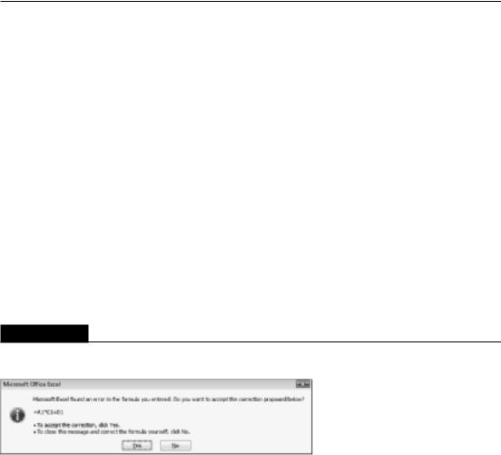
In some cases, if your formula contains mismatched parentheses, Excel may propose a correction to your formula. Figure 10.1 shows an example of the Formula AutoCorrect feature. You may be tempted simply to accept the proposed correction, but be careful — in many cases, the proposed formula, although syntactically correct, isn’t the formula you intended, and it will produce an incorrect result. n

FIGURE 10.1

The Excel Formula AutoCorrect feature sometimes suggests a syntactically correct formula, but not the formula you had in mind.

Tip

Excel lends a hand in helping you match parentheses. When the insertion point moves over a parenthesis while you’re editing a cell, Excel momentarily makes the parenthesis character bold and displays it in a different color — and does the same with its matching parenthesis. n

Using functions in your formulas

Many formulas you create use worksheet functions. These functions enable you to greatly enhance the power of your formulas and perform calculations that are difficult (or even impossible) if you use only the operators discussed previously. For example, you can use the TAN function to calculate the tangent of an angle. You can’t do this complicated calculation by using the mathematical operators alone.

199

Part II: Working with Formulas and Functions

Examples of formulas that use functions

A worksheet function can simplify a formula significantly.

Here’s an example. To calculate the average of the values in 10 cells (A1:A10) without using a function, you’d have to construct a formula like this:

=(A1+A2+A3+A4+A5+A6+A7+A8+A9+A10)/10

Not very pretty, is it? Even worse, you would need to edit this formula if you added another cell to the range. Fortunately, you can replace this formula with a much simpler one that uses one of Excel’s built-in worksheet functions, AVERAGE:

=AVERAGE(A1:A10)

The following formula demonstrates how using a function can enable you to perform calculations that are not otherwise possible. Say you need to determine the largest value in a range. A formula can’t tell you the answer without using a function. Here’s a formula that uses the MAX function to return the largest value in the range A1:D100:

=MAX(A1:D100)

Functions also can sometimes eliminate manual editing. Assume that you have a worksheet that contains 1,000 names in cells A1:A1000, and the names appear in all-capital letters. Your boss sees the listing and informs you that the names will be mail-merged with a form letter. All-uppercase letters is not acceptable; for example, JOHN F. SMITH must now appear as John F. Smith. You could spend the next several hours re-entering the list — ugh — or you could use a formula, such as the following, which uses the PROPER function to convert the text in cell A1 to the proper case:

=PROPER(A1)

Enter this formula once in cell B1 and then copy it down to the next 999 rows. Then select B1:B1000 and choose Home Clipboard Copy to copy the range. Next, with B1:B1000 still selected, choose Home Clipboard Paste Values (V) to convert the formulas to values. Delete the original column, and you’ve just accomplished several hours of work in less than a minute.

One last example should convince you of the power of functions. Suppose you have a worksheet that calculates sales commissions. If the salesperson sold more than $100,000 of product, the commission rate is 7.5 percent; otherwise, the commission rate is 5.0 percent. Without using a function, you would have to create two different formulas and make sure that you use the correct formula for each sales amount. A better solution is to write a formula that uses the IF function to ensure that you calculate the correct commission, regardless of sales amount:

=IF(A1<100000,A1*5%,A1*7.5%)

This formula performs some simple decision-making. The formula checks the value of cell A1. If this value is less than 100,000, the formula returns cell A1 multiplied by 5 percent. Otherwise, it returns what’s in cell A1, multiplied by 7.5 percent. This example uses three arguments, separated by commas. I discuss this in the upcoming section, “Function arguments.”

200

Chapter 10: Introducing Formulas and Functions

New Functions in Excel 2010

New Feature

Excel 2010 contains more than 50 new worksheet functions. n

But, before you get too excited, understand that nearly all the new functions are simply improved versions of existing statistical functions. For example, you’ll find five new functions that deal with the Chi Square distribution: CHISQ.DIST, CHISQ.DIST.RT, CHISQ.INV, CHISQ.INV.RT, and CHISQ. TEST. These are very specialized functions, and the average Excel user will have no need for them.

Excel 2010 offers only three new functions that might appeal to a more general audience:

•AGGREGATE: A function that calculates sums, averages, and so on, with the ability to ignore errors and/or hidden rows.

•NETWORKDAYS.INTL: An international version of the NETWORKDAYS function, which returns the number of workdays between two dates.

•WORKDAY.INTL: An international version of the WORKDAY function, which returns a date before or after a specified number of workdays.

Keep in mind that if you use any of these new functions, you can’t share your workbook with someone who uses an earlier version of Excel.

Function arguments

In the preceding examples, you may have noticed that all the functions used parentheses. The information inside the parentheses is the list of arguments.

Functions vary in how they use arguments. Depending on what it has to do, a function may use

•No arguments

•One argument

•A fixed number of arguments

•An indeterminate number of arguments

•Optional arguments

An example of a function that doesn’t use an argument is the NOW function, which returns the current date and time. Even if a function doesn’t use an argument, you must still provide a set of empty parentheses, like this:

=NOW()

If a function uses more than one argument, you must separate each argument with a comma. The examples at the beginning of the chapter used cell references for arguments. Excel is quite flexible when it comes to function arguments, however. An argument can consist of a cell reference, literal

201