CHAPTER

Performing

Spreadsheet What-If

Analysis

A What-If Example

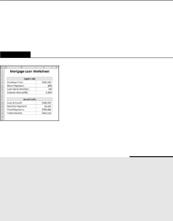
Figure 36.1 shows a simple worksheet model that calculates information pertaining to a mortgage loan. The worksheet is divided into two sections: the input cells and the result cells (which contain formulas).

On the CD

This workbook is available on the companion CD-ROM. The filename is mortgage loan.xlsx.

745

Part V: Analyzing Data with Excel

With this worksheet, you can easily answer the following what-if questions:

•What if I can negotiate a lower purchase price on the property?

•What if the lender requires a 20-percent down payment?

•What if I can get a 40-year mortgage?

•What if the interest rate increases to 7.0 percent?

FIGURE 36.1

This simple worksheet model uses four input cells to produce the results.

You can answer these questions by simply changing the values in the cells in range C4:C7 and observing the effects in the dependent cells (C10:C13). You can, of course, vary any number of input cells simultaneously.

Avoid Hard-Coding Values in a Formula

The mortgage calculation example, simple as it is, demonstrates an important point about spreadsheet design: You should always set up your worksheet so that you have maximum flexibility to make changes. Perhaps the most fundamental rule of spreadsheet design is the following:

Do not hard-code values in a formula. Rather, store the values in separate cells and use cell references in the formula.

The term hard-code refers to the use of actual values, or constants, in a formula. In the mortgage loan example, all the formulas use references to cells, not actual values.

You could use the value 360, for example, for the loan term argument of the pmt function in cell C11 of Figure 36.1. Using a cell reference has two advantages. First, you have no doubt about the values that the formula uses (they aren’t buried in the formula). Second, you can easily change the value — which is easier than editing the formula.

746

Chapter 36: Performing Spreadsheet What-If Analysis

Using values in formulas may not seem like much of an issue when only one formula is involved, but just imagine what would happen if this value were hard-coded into several hundred formulas that were scattered throughout a worksheet.

Types of What-If Analyses

Not surprisingly, Excel can handle much more sophisticated models than the preceding example. To perform a what-if analysis using Excel, you have three basic options:

•Manual what-if analysis: Plug in new values and observe the effects on formula cells.

•Data tables: Create a special type of table that displays the results of selected formula cells as you systematically change one or two input cells.

•Scenario Manager: Create named scenarios and generate reports that use outlines or pivot tables.

I discuss each of these types of what-if analysis in the rest of this chapter.

Manual What-If Analysis

A manual what-if analysis doesn’t require too much explanation. In fact, the example that opens this chapter demonstrates how it’s done. Manual what-if analysis is based on the idea that you have one or more input cells that affect one or more key formula cells. You change the value in the input cells and see what happens to the formula cells. You may want to print the results or save each scenario to a new workbook. The term scenario refers to a specific set of values in one or more input cells.

Manual what-if analysis is very common, and people often use this technique without even realizing that they’re doing a type of what-if analysis. This method of performing what-if analysis certainly has nothing wrong with it, but you should be aware of some other techniques.

Tip

If your input cells are not located near the formula cells, consider using a Watch Window to monitor the formula results in a movable window. I discuss this feature in Chapter 3. n

Creating Data Tables

This section describes one of Excel’s most underutilized features: data tables. A data table is a dynamic range that summarizes formula cells for varying input cells. You can create a data table

747

Part V: Analyzing Data with Excel

fairly easily, but data tables have some limitations. In particular, a data table can deal with only one or two input cells at a time. This limitation becomes clear as you view the examples.

Note

Scenario Manager, discussed later in this chapter (see “Using Scenario Manager”), can produce a report that summarizes any number of input cells and result cells. n

Don’t confuse a data table with a standard table (created by choosing Insert Tables Table). These two features are completely independent.

Creating a one-input data table

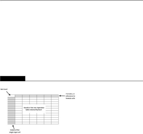
A one-input data table displays the results of one or more formulas for various values of a single input cell. Figure 36.2 shows the general layout for a one-input data table. You need to set up the table yourself, manually. This is not something that Excel will do for you.

FIGURE 36.2

How a one-input data table is set up.

You can place the data table anywhere in a worksheet. The left column contains various values for the single input cell. The top row contains references to formulas located elsewhere in the worksheet. You can use a single formula reference or any number of formula references. The upper-left cell of the table remains empty. Excel calculates the values that result from each value of the input cell and places them under each formula reference.

This example uses the mortgage loan worksheet from earlier in the chapter (see “A What-If Example”). The goal of this exercise is to create a data table that shows the values of the four formula cells (loan amount, monthly payment, total payments, and total interest) for various interest rates ranging from 6 to 8 percent, in 0.25-percent increments.

748

Chapter 36: Performing Spreadsheet What-If Analysis

On the CD

This workbook is available on the companion CD-ROM. The file is named mortgage loan data table.xlsx.

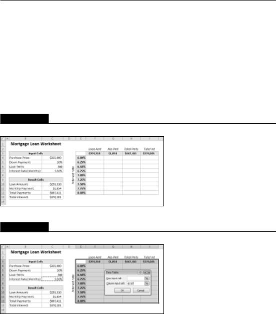
Figure 36.3 shows the setup for the data table area. Row 3 consists of references to the formulas in the worksheet. For example, cell F3 contains the formula =C10, and cell G3 contains the formula =C11. Row 2 contains optional descriptive labels, and these are not actually part of the data table. Column E contains the values of the single input cell (interest rate) that Excel will use in the table.

To create the table, select the data table range (in this case, E3:I12) and then choose Data Data Tools What-If Analysis Data Table. Excel displays the Data Table dialog box, shown in Figure 36.4.

FIGURE 36.3

Preparing to create a one-input data table.

FIGURE 36.4

The Data Table dialog box.

You must specify the worksheet cell that contains the input value. Because variables for the input cell appear in the left column in the data table, you place this cell reference in the Column Input Cell field. Enter C7 or point to the cell in the worksheet. Leave the Row Input Cell field blank.

Click OK, and Excel fills in the table with the calculated results (see Figure 36.5).

749

Part V: Analyzing Data with Excel

FIGURE 36.5

The result of the one-input data table.

Using this table, you can now see the calculated loan values for varying interest rates. If you examine the contents of the cells that Excel entered as a result of this command, you’ll see that the data is generated with a multicell array formula:

{=TABLE(,C7)}

As I discuss in Chapter 16, an array formula is a single formula that can produce results in multiple cells. Because the table uses formulas, Excel updates the table that you produce if you change the cell references in the first row or plug in different interest rates in the first column.

Note

You can arrange a one-input table vertically (as in this example) or horizontally. If you place the values of the input cell in a row, you enter the input cell reference in the Row Input Cell field of the Data Table dialog box. n

Creating a two-input data table

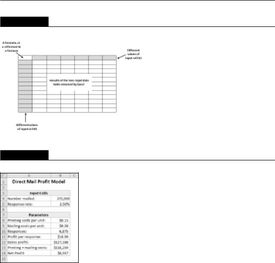
As the name implies, a two-input data table lets you vary two input cells. You can see the setup for this type of table in Figure 36.6. Although it looks similar to a one-input table, the two-input table has one critical difference: It can show the results of only one formula at a time. With a one-input table, you can place any number of formulas, or references to formulas, across the top row of the table. In a two-input table, this top row holds the values for the second input cell. The upper-left cell of the table contains a reference to the single result formula.

Using the mortgage loan worksheet, you could create a two-input data table that shows the results of a formula (say, monthly payment) for various combinations of two input cells (such as interest rate and down-payment percent). To see the effects on other formulas, you simply create multiple data tables — one for each formula cell that you want to summarize.

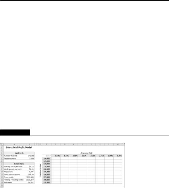
The example in this section uses the worksheet shown in Figure 36.7 to demonstrate a two-input data table. In this example, a company wants to conduct a direct-mail promotion to sell its product. The worksheet calculates the net profit from the promotion.

750

Chapter 36: Performing Spreadsheet What-If Analysis

FIGURE 36.6

The setup for a two-input data table.

FIGURE 36.7

This worksheet calculates the net profit from a direct-mail promotion.

On the CD

This workbook, named direct mail.xlsx, is available on the companion CD-ROM. n

This model uses two input cells: the number of promotional pieces mailed and the anticipated response rate. The following items appear in the Parameters area:

•Printing costs per unit: The cost to print a single mailer. The unit cost varies with the quantity: $0.20 each for quantities less than 200,000; $0.15 each for quantities of 200,001 through 300,000; and $0.10 each for quantities of more than 300,000. The following formula is used:

=IF(B4<200000,0.2,IF(B4<300000,0.15,0.1))

751

Part V: Analyzing Data with Excel

•Mailing costs per unit: A fixed cost, $0.28 per unit mailed.

•Responses: The number of responses, calculated from the response rate and the number mailed. The formula in this cell is the following:

=B4*B5

•Profit per response: A fixed value. The company knows that it will realize an average profit of $18.50 per order.

•Gross profit: This is a simple formula that multiplies the profit-per-response by the number of responses:

=B10*B11

•Print + mailing costs: This formula calculates the total cost of the promotion:

=B4*(B8+B9)

•Net Profit: This formula calculates the bottom line — the gross profit minus the printing and mailing costs.

If you enter values for the two input cells, you see that the net profit varies quite a bit, often going negative to produce a net loss.

Figure 36.8 shows the setup of a two-input data table that summarizes the net profit at various combinations of quantity and response rate; the table appears in the range E4:M14. Cell E4 contains a formula that references the Net Profit cell:

=B14

FIGURE 36.8

Preparing to create a two-input data table.

To create the data table

1.Enter the response rate values in F4:M4.

2.Enter the number mailed values in E5:E14.

752