Part I: Getting Started with Excel

Entering Text and Values into Your Worksheets

To enter a numeric value into a cell, move the cell pointer to the appropriate cell, type the value, and then press Enter or one of the navigation keys. The value is displayed in the cell and also appears in the Formula bar when the cell is selected. You can include decimal points and currency symbols when entering values, along with plus signs, minus signs, and commas (to separate thousands).

Note

If you precede a value with a minus sign or enclose it in parentheses, Excel considers it to be a negative number. n

Entering text into a cell is just as easy as entering a value: Activate the cell, type the text, and then press Enter or a navigation key. A cell can contain a maximum of about 32,000 characters — more than enough to hold a typical chapter in this book. Even though a cell can hold a huge number of characters, you’ll find that it’s not possible to actually display all these characters.

Tip

If you type an exceptionally long text entry into a cell, the Formula bar may not show all the text. To display more of the text in the Formula bar, click the bottom of the Formula bar and drag down to increase the height (see Figure 2.2). Also useful is the Ctrl+Shift+U keyboard shortcut. Pressing this key combination toggles the height of the formula bar to show either one row, or the previous size. n

What happens when you enter text that’s longer than its column’s current width? If the cells to the immediate right are blank, Excel displays the text in its entirety, appearing to spill the entry into adjacent cells. If an adjacent cell isn’t blank, Excel displays as much of the text as possible. (The full text is contained in the cell; it’s just not displayed.) If you need to display a long text string in a cell that’s adjacent to a nonblank cell, you can take one of several actions:

•Edit your text to make it shorter.

•Increase the width of the column (drag the border in the column letter display).

•Use a smaller font.

•Wrap the text within the cell so that it occupies more than one line. Choose Home Alignment Wrap Text to toggle wrapping on and off for the selected cell or range.

32

Chapter 2: Entering and Editing Worksheet Data

FIGURE 2.2

The Formula bar, expanded in height to show more information in the cell.

Entering Dates and Times into Your Worksheets

Excel treats dates and times as special types of numeric values. Typically, these values are formatted so that they appear as dates or times because we humans find it far easier to understand these values when they appear in the correct format. If you work with dates and times, you need to understand Excel’s date and time system.

Entering date values

Excel handles dates by using a serial number system. The earliest date that Excel understands is January 1, 1900. This date has a serial number of 1. January 2, 1900, has a serial number of 2, and so on. This system makes it easy to deal with dates in formulas. For example, you can enter a formula to calculate the number of days between two dates.

33

Part I: Getting Started with Excel

Most of the time, you don’t have to be concerned with Excel’s serial number date system. You can simply enter a date in a familiar date format, and Excel takes care of the details behind the scenes. For example, if you need to enter June 1, 2001, you can simply enter the date by typing June 1, 2001 (or use any of several different date formats). Excel interprets your entry and stores the value 39234, which is the serial number for that date.

Note

The date examples in this book use the U.S. English system. Depending on your Windows regional settings, entering a date in a format (such as June 1, 2011) may be interpreted as text rather than a date. In such a case, you need to enter the date in a format that corresponds to your regional date settings — for example, 1 June, 2011. n

Cross-Reference

For more information about working with dates, see Chapter 12. n

Entering time values

When you work with times, you simply extend Excel’s date serial number system to include decimals. In other words, Excel works with times by using fractional days. For example, the date serial number for June 1, 2011, is 40695. Noon on June 1, 2011 (halfway through the day), is represented internally as 40695.5 because the time fraction is added to the date serial number to get the full date/time serial number.

Again, you normally don’t have to be concerned with these serial numbers (or fractional serial numbers, for times). Just enter the time into a cell in a recognized format.

Cross-Reference

See Chapter 12 for more information about working with time values. n

Modifying Cell Contents

After you enter a value or text into a cell, you can modify it in several ways:

•Erase the cell’s contents.

•Replace the cell’s contents with something else.

•Edit the cell’s contents.

Note

You can also modify a cell by changing its formatting. However, formatting a cell affects only a cell’s appearance. Formatting does not affect its contents. Later sections in this chapter cover formatting. n

34

Chapter 2: Entering and Editing Worksheet Data

Erasing the contents of a cell

To erase the contents of a cell, just click the cell and press Delete. To erase more than one cell, select all the cells that you want to erase and then press Delete. Pressing Delete removes the cell’s contents but doesn’t remove any formatting (such as bold, italic, or a different number format) that you may have applied to the cell.

For more control over what gets deleted, you can choose Home Editing Clear. This command’s drop-down list has five choices:

•Clear All: Clears everything from the cell — its contents, its formatting, and its cell comment (if it has one).

•Clear Formats: Clears only the formatting and leaves the value, text, or formula.

•Clear Contents: Clears only the cell’s contents and leaves the formatting.

•Clear Comments: Clears the comment (if one exists) attached to the cell.

•Clear Hyperlinks: Removes hyperlinks contained in the selected cells. The text remains, but the cell no longer functions as a clickable hyperlink.

Note

Clearing formats doesn’t clear the background colors in a range that has been designated as a table unless you replace the table style background colors manually. n

Replacing the contents of a cell

To replace the contents of a cell with something else, just activate the cell and type your new entry, which replaces the previous contents. Any formatting applied to the cell remains in place and is applied to the new content.

Tip

You can also replace cell contents by dragging and dropping or by pasting data from the Clipboard. In both cases, the cell formatting will be replaced by the format of the new data. To avoid pasting formatting, choose Home Clipboard Paste Values (V), or Home Clipboard Paste Formulas (F). n

Editing the contents of a cell

If the cell contains only a few characters, replacing its contents by typing new data usually is easiest. However, if the cell contains lengthy text or a complex formula and you need to make only a slight modification, you probably want to edit the cell rather than re-enter information.

When you want to edit the contents of a cell, you can use one of the following ways to enter celledit mode.

35

Part I: Getting Started with Excel

•Double-click the cell to edit the cell contents directly in the cell.

•Select the cell and press F2 to edit the cell contents directly in the cell.

•Select the cell that you want to edit and then click inside the Formula bar to edit the cell contents in the Formula bar.

You can use whichever method you prefer. Some people find editing directly in the cell easier; others prefer to use the Formula bar to edit a cell.

Note

The Advanced tab of the Excel Options dialog box contains a section called Editing Options. These settings affect how editing works. (To access this dialog box, choose File Options.) If the Allow Editing Directly in

Cells option isn’t enabled, you can’t edit a cell by double-clicking. In addition, pressing F2 allows you to edit the cell in the Formula bar (not directly in the cell). n

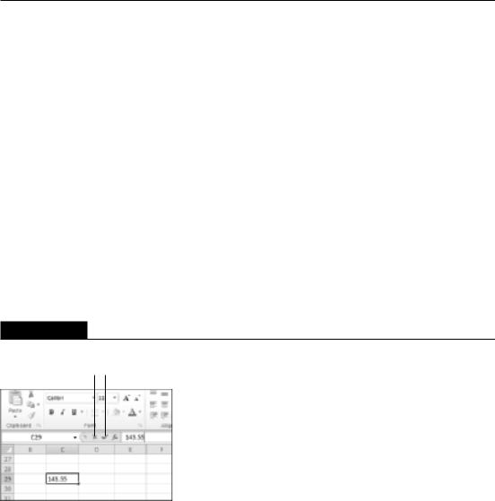
All these methods cause Excel to go into edit mode. (The word Edit appears at the left side of the status bar at the bottom of the screen.) When Excel is in edit mode, the Formula bar displays two new icons: the X and the Check Mark (see Figure 2.3). Clicking the X icon cancels editing without changing the cell’s contents. (Pressing Esc has the same effect.) Clicking the Check Mark icon completes the editing and enters the modified contents into the cell. (Pressing Enter has the same effect.)

FIGURE 2.3

While editing a cell, the Formula bar displays two new icons.

The X icon The Check Mark icon

When you begin editing a cell, the insertion point appears as a vertical bar, and you can perform the following tasks:

•Add new characters at the location of the insertion point. Move the insertion point by • Using the navigation keys to move within the cell

• Pressing Home to move the insertion point to the beginning of the cell • Pressing End to move the insertion point to the end of the cell

36

Chapter 2: Entering and Editing Worksheet Data

•Select multiple characters. Press Shift while you use the navigation keys.

•Select characters while you’re editing a cell. Use the mouse. Just click and drag the mouse pointer over the characters that you want to select.

Learning some handy data-entry techniques

You can simplify the process of entering information into your Excel worksheets and make your work go quite a bit faster by using a number of useful tricks, described in the following sections.

Automatically moving the cell pointer after entering data

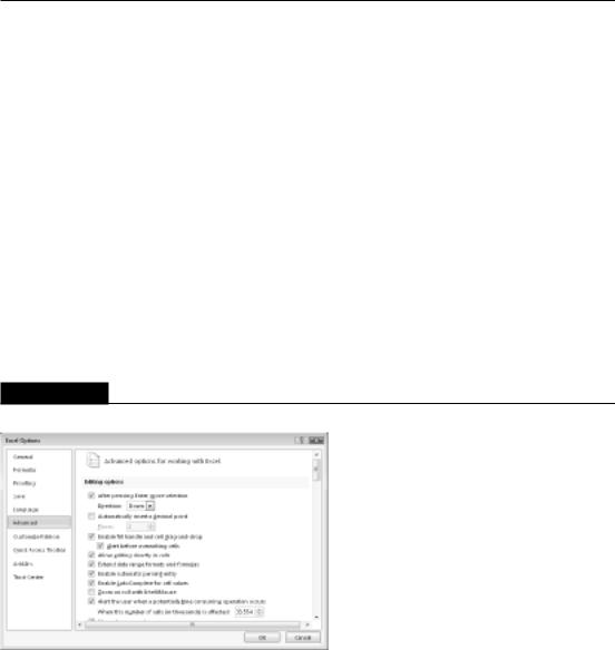
By default, Excel automatically moves the cell pointer to the next cell down when you press the Enter key after entering data into a cell. To change this setting, choose File Options and click the Advanced tab (see Figure 2.4). The check box that controls this behavior is labeled After Pressing Enter, Move Selection. If you enable this option, you can choose the direction in which the cell pointer moves (down, left, up, or right).

Your choice is completely a matter of personal preference. I prefer to keep this option turned off. When entering data, I use the navigation keys rather than the Enter key (see the next section).

FIGURE 2.4

You can use the Advanced tab in Excel Options to select a number of helpful input option settings.

Using navigation keys instead of pressing Enter

Instead of pressing the Enter key when you’re finished making a cell entry, you also can use any of the navigation keys to complete the entry. Not surprisingly, these navigation keys send you in the direction that you indicate. For example, if you’re entering data in a row, press the rightarrow (→) key rather than Enter. The other arrow keys work as expected, and you can even use PgUp and PgDn.

37

Part I: Getting Started with Excel

Selecting a range of input cells before entering data

Here’s a tip that most Excel users don’t know about: When a range of cells is selected, Excel automatically moves the cell pointer to the next cell in the range when you press Enter. If the selection consists of multiple rows, Excel moves down the column; when it reaches the end of the selection in the column, it moves to the first selected cell in the next column.

To skip a cell, just press Enter without entering anything. To go backward, press Shift+Enter. If you prefer to enter the data by rows rather than by columns, press Tab rather than Enter. Excel continues to cycle through the selected range until you select a cell outside of the range.

Using Ctrl+Enter to place information into multiple cells simultaneously

If you need to enter the same data into multiple cells, Excel offers a handy shortcut. Select all the cells that you want to contain the data, enter the value, text, or formula, and then press Ctrl+Enter. The same information is inserted into each cell in the selection.

Entering decimal points automatically

If you need to enter lots of numbers with a fixed number of decimal places, Excel has a useful tool that works like some adding machines. Access the Excel Options dialog box and click the Advanced tab. Select the check box Automatically Insert a Decimal Point and make sure that the Places box is set for the correct number of decimal places for the data you need to enter.

When this option is set, Excel supplies the decimal points for you automatically. For example, if you specify two decimal places, entering 12345 into a cell is interpreted as 123.45. To restore things to normal, just clear the Automatically Insert a Decimal Point check box in the Excel Options dialog box. Changing this setting doesn’t affect any values that you already entered.

Caution

The fixed decimal–places option is a global setting and applies to all workbooks (not just the active workbook). If you forget that this option is turned on, you can easily end up entering incorrect values — or cause some major confusion if someone else uses your computer. n

Using AutoFill to enter a series of values

The Excel AutoFill feature makes inserting a series of values or text items in a range of cells easy. It uses the AutoFill handle (the small box at the lower right of the active cell). You can drag the AutoFill handle to copy the cell or automatically complete a series.

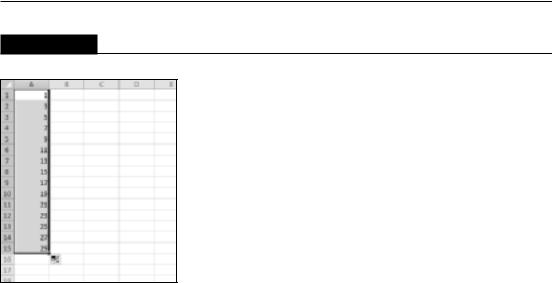
Figure 2.5 shows an example. I entered 1 into cell A1 and 3 into cell A2. Then I selected both cells and dragged down the fill handle to create a linear series of odd numbers. The figure also shows a Smart Icon that, when clicked, displays some additional AutoFill options.

Tip

If you drag the AutoFill handle while you press and hold the right mouse button, Excel displays a shortcut menu with additional fill options. n

38

Chapter 2: Entering and Editing Worksheet Data

FIGURE 2.5

This series was created by using AutoFill.

Using AutoComplete to automate data entry

The Excel AutoComplete feature makes entering the same text into multiple cells easy. With AutoComplete, you type the first few letters of a text entry into a cell, and Excel automatically completes the entry based on other entries that you already made in the column. Besides reducing typing, this feature also ensures that your entries are spelled correctly and are consistent.

Here’s how it works. Suppose that you’re entering product information in a column. One of your products is named Widgets. The first time that you enter Widgets into a cell, Excel remembers it. Later, when you start typing Widgets in that same column, Excel recognizes it by the first few letters and finishes typing it for you. Just press Enter, and you’re done. To override the suggestion, just keep typing.

AutoComplete also changes the case of letters for you automatically. If you start entering widget (with a lowercase w) in the second entry, Excel makes the w uppercase to be consistent with the previous entry in the column.

Tip

You also can access a mouse-oriented version of AutoComplete by right-clicking the cell and choosing Pick from Drop-Down List from the shortcut menu. Excel then displays a drop-down box that has all the entries in the current column, and you just click the one that you want. n

Keep in mind that AutoComplete works only within a contiguous column of cells. If you have a blank row, for example, AutoComplete identifies only the cell contents below the blank row.

If you find the AutoComplete feature distracting, you can turn it off by using the Advanced tab of the Excel Options dialog box. Remove the check mark from the check box labeled Enable AutoComplete for Cell Values.

39

Part I: Getting Started with Excel

Forcing text to appear on a new line within a cell

If you have lengthy text in a cell, you can force Excel to display it in multiple lines within the cell: Press Alt+Enter to start a new line in a cell.

Note

When you add a line break, Excel automatically changes the cell’s format to Wrap Text. But unlike normal text wrap, your manual line break forces Excel to break the text at a specific place within the text, which gives you more precise control over the appearance of the text than if you rely on automatic text wrapping. n

Tip

To remove a manual line break, edit the cell and press Delete when the insertion point is located at the end of the line that contains the manual line break. You won’t see any symbol to indicate the position of the manual line break, but the text that follows it will move up when the line break is deleted. n

Using AutoCorrect for shorthand data entry

You can use the AutoCorrect feature to create shortcuts for commonly used words or phrases. For example, if you work for a company named Consolidated Data Processing Corporation, you can create an AutoCorrect entry for an abbreviation, such as cdp. Then, whenever you type cdp, Excel automatically changes it to Consolidated Data Processing Corporation.

Excel includes quite a few built-in AutoCorrect terms (mostly common misspellings), and you can add your own. To set up your custom AutoCorrect entries, access the Excel Options dialog box (choose File Options) and click the Proofing tab. Then click the AutoCorrect Options button to display the AutoCorrect dialog box. In the dialog box, click the AutoCorrect tab, check the option labeled Replace Text as You Type, and then enter your custom entries. (Figure 2.6 shows an example.) You can set up as many custom entries as you like. Just be careful not to use an abbreviation that might appear normally in your text.

Tip

Excel shares your AutoCorrect list with other Office applications. For example, any AutoCorrect entries you created in Word also work in Excel. n

Entering numbers with fractions

To enter a fractional value into a cell, leave a space between the whole number and the fraction. For example, to enter 67⁄8, enter 6 7/8 and then press Enter. When you select the cell, 6.875 appears in the Formula bar, and the cell entry appears as a fraction. If you have a fraction only (for example, 1⁄8), you must enter a zero first, like this — 0 1/8 — or Excel will likely assume that you’re entering a date. When you select the cell and look at the Formula bar, you see 0.125. In the cell, you see 1⁄8.

Simplifying data entry by using a form

Many people use Excel to manage lists in which the information is arranged in rows. Excel offers a simple way to work with this type of data through the use of a data entry form that Excel can create automatically. This data form works with either a normal range of data, or with a range that has been designated as a table (choose Insert Tables Table). Figure 2.7 shows an example.

40

Chapter 2: Entering and Editing Worksheet Data

FIGURE 2.6

AutoCorrect allows you to create shorthand abbreviations for text you enter often.

Unfortunately, the command to access the data form is not on the Ribbon. To use the data form, you must add it to your Quick Access toolbar or add it to the Ribbon. The instructions that follow describe how to add this command to your Quick Access toolbar:

1.Right-click the Quick Access toolbar and choose Customize Quick Access Toolbar.

The Quick Access Toolbar panel of the Excel Options dialog box appears.

2.In the Choose Commands From drop-down list, choose Commands Not in the Ribbon.

3.In the list box on the left, select Form.

4.Click the Add button to add the selected command to your Quick Access toolbar.

5.Click OK to close the Excel Options dialog box.

FIGURE 2.7

Excel’s built-in data form can simplify many data-entry tasks.

41