


Chapter 5: Introducing Tables
The range is converted to a table (using the default table style), and the Table Tools Design tab of the Ribbon appears.
Note
Excel may guess the table’s dimensions incorrectly if the table isn’t separated from other information by at least one empty row or column. If Excel guesses incorrectly, just specify the exact range for the table in the Create Table dialog box. Better yet, click Cancel and rearrange your worksheet such that the table is separated from your other data by at least one blank row or column. n
To create a table from an empty range, just select the range and choose Insert Tables Table. Excel creates the table, adds generic column headers (such as Column1 and Column2), and applies table formatting to the range.
Changing the Look of a Table
When you create a table, Excel applies the default table style. The actual appearance depends on which document theme is used in the workbook. If you prefer a different look, you can easily change the entire look of the table.
Select any cell in the table and choose Table Tools Design Table Styles. The Ribbon shows one row of styles, but if you click the bottom of the scrollbar to the right, the table styles group expands, as shown in Figure 5.5. The styles are grouped into three categories: Light, Medium, and Dark. Notice that you get a “live” preview as you move your mouse among the styles. When you see one you like, just click to make it permanent. And yes, some are really ugly and practically illegible.
For a different set of color choices, choose Page Layout Themes Themes to select a different document theme. For more information about themes, see Chapter 6.
Tip
If applying table styles isn’t working, it’s probably because the range was already formatted before you converted it to a table. Table formatting doesn’t override normal formatting. To clear existing background fill colors, select the entire table and choose Home Font Fill Color No Fill. To clear existing font colors, choose Home Font Font Color Automatic. To clear existing borders, choose Home Font Borders No Borders. After you issue these commands, the table styles should work as expected. n
If you’d like to create a custom table style, choose Table Tools Design Table Styles New Table Style to display the New Table Quick Style dialog box shown in Figure 5.6. You can customize any or all of the 12 table elements. Select an element from the list, click Format, and specify the formatting for that element. When you’re finished, give the new style a name and click OK. Your custom table style will appear in the Table Styles gallery in the Custom category. Unfortunately, custom table styles are available only in the workbook in which they were created.
103

Part I: Getting Started with Excel
FIGURE 5.5
Excel offers many different table styles.
FIGURE 5.6
Use this dialog box to create a new table style.
104
Chapter 5: Introducing Tables
Tip
If you would like to make changes to an existing table style, locate it in the Ribbon and right-click. Choose Duplicate from the shortcut menu. Excel displays the Modify Table Quick Style dialog box with all the settings from the specified table style. Make your changes, give the style a new name, and click OK to save it as a custom table style. n
Working with Tables
This section describes some common actions you’ll take with tables.
Navigating in a table
Selecting cells in a table works just like selecting cells in a normal range. One difference is when you use the Tab key. Pressing Tab moves to the cell to the right, and when you reach the last column, pressing Tab again moves to the first cell in the next row.
Selecting parts of a table
When you move your mouse around in a table, you may notice that the pointer changes shapes. These shapes help you select various parts of the table.
•To select an entire column: Move the mouse to the top of a cell in the header row, and the mouse pointer changes to a down-pointing arrow. Click to select the data in the column. Click a second time to select the entire table column (including the Header Row and the Total Row, if it has one). You can also press Ctrl+spacebar (once or twice) to select a column.
•To select an entire row: Move the mouse to the left of a cell in the first column, and the mouse pointer changes to a right-pointing arrow. Click to select the entire table row. You can also press Shift+spacebar to select a table row.
•To select the entire table: Move the mouse to the upper-left part of the upper-left cell. When the mouse pointer turns into a diagonal arrow, click to select the data area of the table. Click a second time to select the entire table (including the Header Row and the Total Row). You can also press Ctrl+A (once or twice) to select the entire table.
Tip
Right-clicking a cell in a table displays several selection options in the shortcut menu. n
Adding new rows or columns
To add a new column to the end of a table, select a cell in the column to the right of the table and start entering the data. Excel automatically extends the table horizontally.
105

Part I: Getting Started with Excel
Similarly, if you enter data in the row below a table, Excel extends the table vertically to include the new row.
Note
An exception to automatically extending tables is when the table is displaying a Total Row. If you enter data below the Total Row, the table will not be extended. and the data will not be part of the table. n
To add rows or columns within the table, right-click and choose Insert from the shortcut menu. The Insert shortcut menu command displays additional menu items:
•Table Columns to the Left
•Table Columns to the Right
•Table Rows Above
•Table Rows Below
Tip
When the cell pointer is in the bottom-right cell of a table, pressing Tab inserts a new row at the bottom of the table, above the Total Row (if the table has one). n
When you move your mouse to the resize handle at bottom-right cell of a table, the mouse pointer turns into a diagonal line with two arrow heads. Click and drag down to add more rows to the table. Click and drag to the right to add more columns.
When you insert a new column, the Header Row displays a generic description, such as Column1, Column2, and so on. Typically, you’ll want to change these names to more descriptive labels. Just select the cell and overwrite the generic text with your new text.
Deleting rows or columns
To delete a row (or column) in a table, select any cell in the row (or column) to be deleted. To delete multiple rows or columns, select a range of cells. Then right-click and choose Delete Table Rows (or Delete Table Columns).
Moving a table
To move a table to a new location in the same worksheet, move the mouse pointer to any of its borders. When the mouse pointer turns into a cross with four arrows, click and drag the table to its new location.
To move a table to a different worksheet (which could be in a different workbook), you can drag and drop it as well — as long as the destination worksheet is visible onscreen.
106

Chapter 5: Introducing Tables
Excel Remembers
When you do something with a complete column in a table, Excel remembers that and extends that “something” to all new entries added to that column. For example, if you apply currency formatting to a column and then add a new row, Excel applies currency formatting to the new value in that column.
The same thing applies to other operations, such as conditional formatting, cell protection, data validation, and so on. And if you create a chart using the data in a table, the chart will be extended automatically if you add new data to the table. Those who have used versions prior to Excel 2007 will appreciate this feature the most.
Or, you can use these steps to move a table to different worksheet or workbook:
1.Press Ctrl+A twice to select the entire table.
2.Press Ctrl+X to cut the selected cells.
3.Activate the new worksheet and select the upper-left cell for the table.
4.Press Ctrl+V to paste the table.
Setting table options
The Table Style Options group of the Table Tools Design tab contains several check boxes that determine whether various elements of the table are displayed, and whether some formatting options are in effect:
•Header Row: Toggles the display of the Header Row.
•Total Row: Toggles the display of the Total Row.
•First Column: Toggles special formatting for the first column. Depending on the table style used, this command might have no effect.
•Last Column: Toggles special formatting for the last column. Depending on the table style used, this command might have no effect.
•Banded Rows: Toggles the display of banded (alternating color) rows.
•Banded Columns: Toggles the display of banded columns.
Working with the Total Row
The Total Row in a table contains formulas that summarize the information in the columns. When you create a table, the Total Row isn’t turned on. To display the Total Row, choose Table Tools Design Table Style Options and put a check mark next to Total Row.
107

Part I: Getting Started with Excel
By default, a Total Row displays the sum of the values in a column of numbers. In many cases, you’ll want a different type of summary formula. When you select a cell in the Total Row, a drop-down arrow appears in the cell. Click the arrow, and you can select from a number of other summary formulas (see Figure 5.7):
•None: No formula
•Average: Displays the average of the numbers in the column
•Count: Displays the number of entries in the column (blank cells are not counted)
•Count Numbers: Displays the number of numeric values in the column (blank cells, text cells, and error cells are not counted)
•Max: Displays the maximum value in the column
•Min: Displays the minimum value in the column
•Sum: Displays the sum of the values in the column
•StdDev: Displays the standard deviation of the values in the column. Standard deviation is a statistical measure of how “spread out” the values are.
•Var: Displays the variance of the values in the column. Variance is another statistical measure of how “spread out” the values are.
•More Functions: Displays the Insert Function dialog box so that you can select a function that isn’t in the list.
FIGURE 5.7
Several types of summary formulas are available for the Total Row.
Caution
If you have a formula that refers to a value in the Total Row of a table, the formula returns an error if you hide the Total Row. But if you make the Total Row visible again, the formula works as it should. n
108

Chapter 5: Introducing Tables
Cross-Reference
For more information about formulas, including the use of formulas in a table column, see Chapter 10. n
Removing duplicate rows from a table
If data in a table was obtained from multiple sources, the table may contain duplicate items. Most of the time, you want to eliminate the duplicates. In the past, removing duplicate data was essentially a manual task, but it’s very easy if the data is in a table.
Start by selecting any cell in your table. Then choose Table Tools Design Tools Remove Duplicates. Excel responds with Remove Duplicates dialog box shown in Figure 5.8. The dialog box lists all the columns in your table. Place a check mark next to the columns that you want to be included in the duplicate search. Most of the time, you’ll want to select all the columns, which is the default. Click OK, and Excel weeds out the duplicate rows and displays a message that tells you how many duplicates it removed.
When you select all columns in the Remove Duplicates dialog box, Excel will delete a row only if the content of every column is duplicated. In some situations, you may not care about matching some columns, so you would deselect those columns in the Remove Duplicates dialog box. In the example shown in Figure 5.8, removing the check mark from all columns except Agent would result in a table that showed one row per agent — an unduplicated list of all agents.
FIGURE 5.8
Removing duplicate rows from a table is easy.
Caution
It’s important to understand that duplicate values are determined by the value displayed in the cell — not necessarily the value stored in the cell. For example, assume that two cells contain the same date. One of the dates is formatted to display as 5/15/2011, and the other is formatted to display as May 15, 2011. When removing duplicates, Excel considers these dates to be different. n
109

Part I: Getting Started with Excel
Sorting and filtering a table
The Header Row of a table contains a drop-down arrow that, when clicked, displays sorting and filtering options (see Figure 5.9).
FIGURE 5.9
Each column in a table contains sorting and filtering option.
Sorting a table
Sorting a table rearranges the rows based on the contents of a particular column. You may want to sort a table to put names in alphabetical order. Or, maybe you want to sort your sales staff by the totals sales made.
To sort a table by a particular column, click the drop-down in the column header and choose one of the sort commands. The exact command varies, depending on the type of data in the column.
You can also select Sort by Color to sort the rows based on the background or text color of the data. This option is relevant only if you’ve overridden the table style colors with custom formatting.
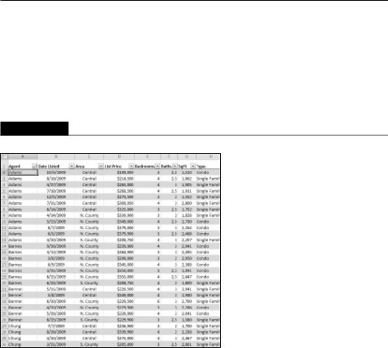
You can sort on any number of columns. The trick is to sort the least significant column first and then proceed until the most significant column is sorted lasted. For example, in the real estate table, you may want to sort the list by agent. And within each agent’s group, sort the rows by area.
110
Chapter 5: Introducing Tables
And within each area, sort the rows by list price. For this type of sort, first sort by the List Price column, then sort by the Area column, and then sort by the Agent column. Figure 5.10 shows the table sorted in this manner.
Note
When a column is sorted, the drop-down list in the header row displays a different graphic to remind you that the table is sorted by that column. n
FIGURE 5.10
A table, after performing a three-column sort.
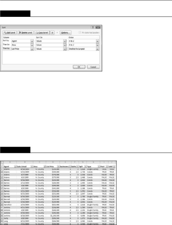
Another way of performing a multiple-column sort is to use the Sort dialog box (choose Home Editing Sort & Filter Custom Sort). Or, right-click any cell in the table and choose Sort Custom Sort from the shortcut menu.
In the Sort dialog box, use the drop-down lists to specify the sort specifications. In this example, you start with Agent. Then, click the Add Level button to insert another set of search controls. In this new set of controls, specify the sort specifications for the Area column. Then, add another level and enter the specifications for the List Price column. Figure 5.11 shows the dialog box after entering the specifications for the three-column sort. This technique produces exactly the same sort as described in the previous paragraph.
111
Part I: Getting Started with Excel
FIGURE 5.11
Using the Sort dialog box to specify a three-column sort.
Filtering a table
Filtering a table refers to displaying only the rows that meet certain conditions. (The other rows are hidden.)
Using the real estate table, assume that you’re only interested in the data for the N. County area. Click the drop-down arrow in the Area Row Header and remove the check mark from Select All, which unselects everything. Then, place a check mark next to N. County and click OK. The table, shown in Figure 5.12, is now filtered to display only the listings in the N. County area. Notice that some of the row numbers are missing; these rows contain the filtered (hidden) data.
Also notice that the drop-down arrow in the Area column now shows a different graphic — an icon that indicates the column is filtered.
FIGURE 5.12
This table is filtered to show only the information for N. County.
112

Chapter 5: Introducing Tables
You can filter by multiple values in a column by using multiple check marks. For example, to filter the table to show only N. County and Central, place a check mark next to both values in the dropdown list in the Area Row Header.
You can filter a table using any number of columns. For example, you may want to see only the N. County listings in which the Type is Single Family. Just repeat the operation using the Type column. All tables then display only the rows in which the Area is N. County and the Type is Single Family.
For additional filtering options, select Text Filters (or Number Filters, if the column contains values). The options are fairly self-explanatory, and you have a great deal of flexibility in displaying only the rows that you’re interested in.
In addition, you can right-click a cell and use the Filter command on the shortcut menu. This menu item leads to several additional filtering options.
Note
As you may expect, the Total Row is updated to show the total only for the visible rows. n
When you copy data from a filtered table, only the visible data is copied. In other words, rows that are hidden by filtering don’t get copied. This filtering makes it very easy to copy a subset of a larger table and paste it to another area of your worksheet. Keep in mind, though, that the pasted data is not a table — it’s just a normal range. You can, however, convert the copied range to a table.
To remove filtering for a column, click the drop-down in the Row Header and select Clear Filter. If you’ve filtered using multiple columns, it may be faster to remove all filters by choosing Home Editing Sort & Filter Clear.
Converting a table back to a range
If you need to convert a table back to a normal range, just select a cell in the table and choose Table Tools Design Tools Convert to Range. The table style formatting remains intact, but the range no longer functions as a table.
113