Chapter 34: Introducing Pivot Tables

Creating a Pivot Table

In this section, I describe the basic steps required to create a pivot table, using the bank account data described earlier in this chapter. Creating a pivot table is an interactive process. It’s not at all uncommon to experiment with various layouts until you find one that you’re satisfied with.

If you’re unfamiliar with the elements of a pivot table, see the upcoming sidebar, “Pivot Table Terminology.”

Specifying the data

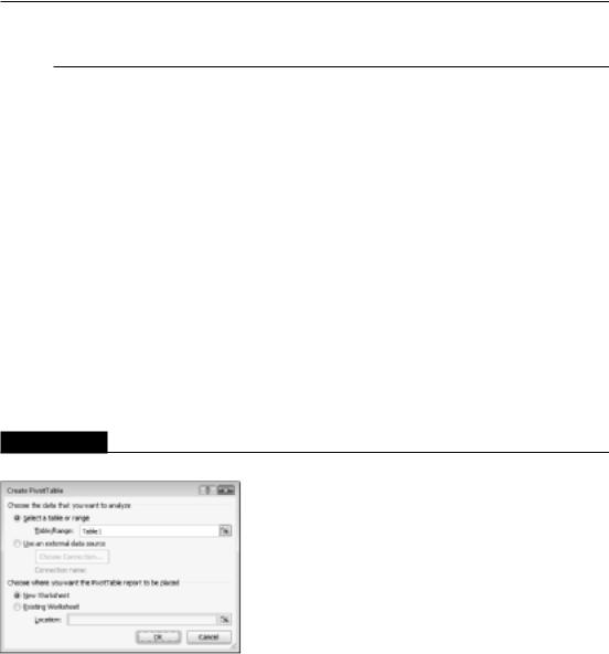
If your data is in a worksheet range, select any cell in that range and then choose Insert Tables PivotTable, which displays the dialog box shown in Figure 34.7.

Excel attempts to guess the range, based on the location of the active cell. If you’re creating a pivot table from an external data source, you need to select that option and then click Choose Connection to specify the data source.

Tip

If you’re creating a pivot table from data in a worksheet, it’s a good idea to first create a table for the range (choose Insert Tables Table). Then, if you expand the table by adding new rows of data, Excel will refresh the pivot table without the need to manually indicate the new data range. n

FIGURE 34.7

In the Create PivotTable dialog box, you tell Excel where the data is and where you want the pivot table.

Specifying the location for the pivot table

Use the bottom section of the Create PivotTable dialog box to indicate the location for your pivot table. The default location is on a new worksheet, but you can specify any range on any worksheet, including the worksheet that contains the data.

701

Part V: Analyzing Data with Excel

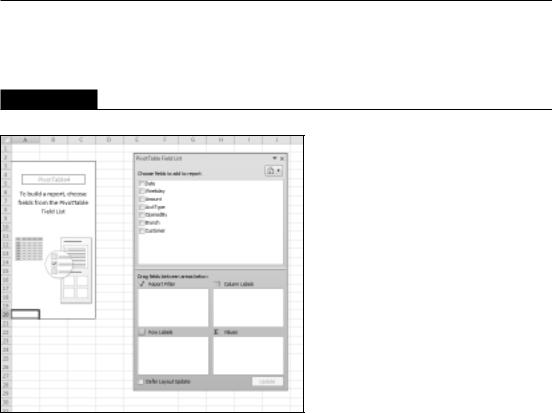
Click OK, and Excel creates an empty pivot table and displays its PivotTable Field List task pane, as shown in Figure 34.8.

FIGURE 34.8

Use the PivotTable Field List to build the pivot table.

Tip

The PivotTable Field List is typically docked on the right side of the Excel window. Drag its title bar to move it anywhere you like. Also, if you click a cell outside the pivot table, the PivotTable Field List is hidden. n

Laying out the pivot table

Next, set up the actual layout of the pivot table. You can do so by using either of any techniques:

•Drag the field names (at the top) to one of the four boxes at the bottom of the PivotTable Field List.

•Place a check mark next to the item at the top of the PivotTable Field List. Excel will place the field into one of the four boxes at the bottom.

•Right-click a field name at the top of the PivotTable Field List and choose its location from the shortcut menu.

702

Chapter 34: Introducing Pivot Tables

Note

In versions prior to Excel 2007, you could drag items from the field list directly into the appropriate area of the pivot table. This feature is still available, but it’s turned off by default. To enable this feature, choose PivotTable Tools Options PivotTable Options Options to display the PivotTable Options dialog box. Click the Display tab and then select the Classic PivotTable Layout check box. n

The following steps create the pivot table presented earlier in this chapter (see “A pivot table example”). For this example, I drag the items from the top of the PivotTable Field List to the areas in the bottom of the PivotTable Field List.

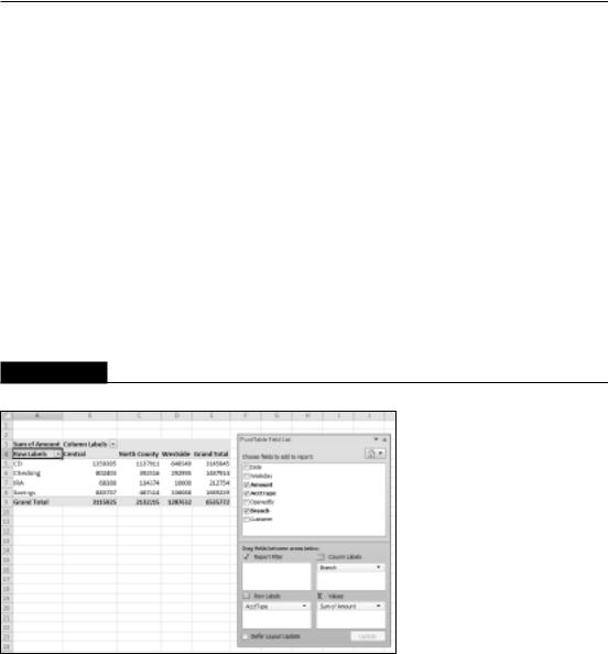
1.Drag the Amount field into the Values area. At this point, the pivot table displays the total of all the values in the Amount column.

2.Drag the AcctType field into the Row Labels area. Now the pivot table shows the total amount for each of the account types.

3.Drag the Branch field into the Column Labels area. The pivot table shows the amount for each account type, cross-tabulated by branch (see Figure 34.9). The pivot table updates itself automatically with every change you make in the PivotTable Field List.

FIGURE 34.9

After a few simple steps, the pivot table shows a summary of the data.

Formatting the pivot table

Notice that the pivot table uses General number formatting. To change the number format for all data, right-click any value and choose Number Format from the shortcut menu. Then use the Format Cells dialog box to change the number format for the displayed data.

703

Part V: Analyzing Data with Excel

You can apply any of several built-in styles to a pivot table. Select any cell in the pivot table and then choose PivotTable Tools Design PivotTable Styles to select a style.

You also can use the controls from the PivotTable Design Layout group to control various elements in the pivot table. For example, you can choose to hide the grand totals if you prefer.

The PivotTable Tools Options Show group contains additional options that affect the appearance of your pivot table. For example, you use the Show Field Headers button to toggle the display of the field headings.

Still more pivot table options are available from the PivotTable Options dialog box, shown in Figure 34.10. To display this dialog box, choose PivotTable Tools Options PivotTable

Options. Or, right-click any cell in the pivot table and choose Table Options from the shortcut menu.

Pivot Table Terminology

Understanding the terminology associated with pivot tables is the first step in mastering this feature. Refer to the accompanying figure to get your bearings.

•Column labels: A field that has a column orientation in the pivot table. Each item in the field occupies a column. In the figure, Customer represents a column field that contains two items (Existing and New). You can have nested column fields.

•Grand totals: A row or column that displays totals for all cells in a row or column in a pivot table. You can specify that grand totals be calculated for rows, columns, or both (or neither). The pivot table in the figure shows grand totals for both rows and columns.

•Group: A collection of items treated as a single item. You can group items manually or automatically (group dates into months, for example). The pivot table in the figure does not have any defined groups.

704

Chapter 34: Introducing Pivot Tables

•Item: An element in a field that appears as a row or column header in a pivot table. In the figure, Existing and New are items for the Customer field. The Branch field has three items: Central, North County, and Westside. AcctType has four items: CD, Checking, IRA, and Savings.

•Refresh: Recalculates the pivot table after making changes to the source data.

•Row labels: A field that has a row orientation in the pivot table. Each item in the field occupies a row. You can have nested row fields. In the figure, Branch and AcctType both represent row fields.

•Source data: The data used to create a pivot table. It can reside in a worksheet or an external database.

•Subtotals: A row or column that displays subtotals for detail cells in a row or column in a pivot table. The pivot table in the figure displays subtotals for each branch.

•Table Filter: A field that has a page orientation in the pivot table — similar to a slice of a three-dimensional cube. You can display only one item (or all items) in a page field at one time. In the figure, OpenedBy represents a page field that displays All (that is, not filtered). In previous version of Excel, a table filter was known as a Page field.

•Values area: The cells in a pivot table that contain the summary data. Excel offers several ways to summarize the data (sum, average, count, and so on).

FIGURE 34.10

The PivotTable Options dialog box.

705

Part V: Analyzing Data with Excel

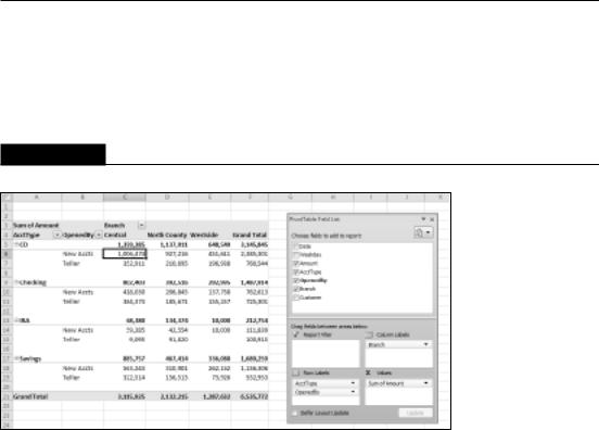
Modifying the pivot table

After you create a pivot table, changing it is easy. For example, you can add further summary information by using the PivotTable Field List. Figure 34.11 shows the pivot table after I dragged a second field (OpenedBy) to the Row Labels section in the PivotTable Field List.

FIGURE 34.11

Two fields are used for row labels.

The following are some tips on other pivot table modifications you can make:

•To remove a field from the pivot table, select it in the bottom part of the PivotTable Field List and then drag it away.

•If an area has more than one field, you can change the order in which the fields are listed by dragging the field names. Doing so affects the appearance of the pivot table.

•To temporarily remove a field from the pivot table, remove the check mark from the field name in the top part of the PivotTable Field List. The pivot table is redisplayed without that field. Place the check mark back on the field name, and it appears in its previous section.

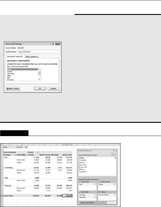
•If you add a field to the Report Filter section, the field items appear in a drop-down list, which allows you to filter the displayed data by one or more items. Figure 34.12 shows an example. I dragged the Date field to the Report Filter area. The report is now showing the data only for a single day (which I selected from the drop-down list in cell B1).

706

Chapter 34: Introducing Pivot Tables

Pivot Table Calculations

Pivot table data is most frequently summarized using a sum. However, you can display your data using a number of different summary techniques. Select any cell in the Values area of your pivot table and then choose PivotTable Tools Options Active Field Field Settings to display the Value Field Settings dialog box. This dialog box has two tabs: Summarize Values By and Show Values As.

Use the Summarize Values By tab to select a different summary function. Your choices are Sum, Count, Average, Max, Min, Product, Count Numbers, StdDev, StdDevp, Var, and Varp.

To display your values in a different form, use the drop-down control on the Show Values As tab. You have many options to choose from, including as a percentage of the total or subtotal.

FIGURE 34.12

The pivot table is filtered by date.

707