Chapter 13: Creating Formulas That Count and Sum

Cross-Reference

I cover pivot tables in detail in Chapters 34 and 35, and you can learn more about the conditional formatting data bars in Chapter 20. n

FIGURE 13.10

Using data bars within a pivot table to display a histogram.

Summing Formulas

The examples in this section demonstrate how to perform common summing tasks by using formulas. The formulas range from very simple to relatively complex array formulas that compute sums by using multiple criteria.

Summing all cells in a range

It doesn’t get much simpler than this. The following formula returns the sum of all values in a range named Data:

=SUM(Data)

The SUM function can take up to 255 arguments. The following formula, for example, returns the sum of the values in five noncontiguous ranges:

=SUM(A1:A9,C1:C9,E1:E9,G1:G9,I1:I9)

299

Part II: Working with Formulas and Functions

You can use complete rows or columns as an argument for the SUM function. The formula that follows, for example, returns the sum of all values in column A. If this formula appears in a cell in column A, it generates a circular reference error.

=SUM(A:A)

The following formula returns the sum of all values on Sheet1 by using a range reference that consists of all rows. To avoid a circular reference error, this formula must appear on a sheet other than Sheet1.

=SUM(Sheet1!1:1048576)

The SUM function is very versatile. The arguments can be numerical values, cells, ranges, text representations of numbers (which are interpreted as values), logical values, and even embedded functions. For example, consider the following formula:

=SUM(B1,5,”6”,,SQRT(4),A1:A5,TRUE)

This odd formula, which is perfectly valid, contains all the following types of arguments, listed here in the order of their presentation:

•A single cell reference: B1

•A literal value: 5

•A string that looks like a value: “6”

•A missing argument: , ,

•An expression that uses another function: SQRT(4)

•A range reference: A1:A5

•A logical value: TRUE

Caution

The SUM function is versatile, but it’s also inconsistent when you use logical values (TRUE or FALSE). Logical values stored in cells are always treated as 0. However, logical TRUE, when used as an argument in the SUM function, is treated as 1.

Computing a cumulative sum

You may want to display a cumulative sum of values in a range — sometimes known as a “running total.” Figure 13.11 illustrates a cumulative sum. Column B shows the monthly amounts, and column C displays the cumulative (year-to-date) totals.

The formula in cell C2 is

=SUM(B$2:B2)

Notice that this formula uses a mixed reference — that is, the first cell in the range reference always refers to the same row (in this case, row 2). When this formula is copied down the column, the

300

Chapter 13: Creating Formulas That Count and Sum

range argument adjusts such that the sum always starts with row 2 and ends with the current row. For example, after copying this formula down column C, the formula in cell C8 is

=SUM(B$2:B8)

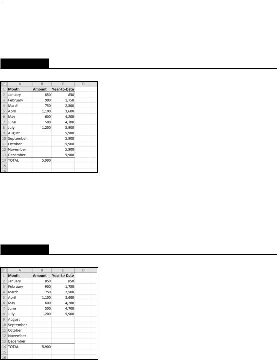
FIGURE 13.11

Simple formulas in column C display a cumulative sum of the values in column B.

You can use an IF function to hide the cumulative sums for rows in which data hasn’t been entered. The following formula, entered in cell C2 and copied down the column, is

=IF(B2<>””,SUM(B$2:B2),””)

Figure 13.12 shows this formula at work.

FIGURE 13.12

Using an IF function to hide cumulative sums for missing data.

301

Part II: Working with Formulas and Functions

On the CD

This workbook is available on the companion CD-ROM. The file is named cumulative sum.xlsx.

Summing the “top n” values

In some situations, you may need to sum the n largest values in a range — for example, the top ten values. If your data resides in a table, you can use autofiltering to hide all but the top n rows and then display the sum of the visible data in the table’s total row.

Another approach is to sort the range in descending order and then use the SUM function with an argument consisting of the first n values in the sorted range.

A better solution — which doesn’t require a table or sorting — uses an array formula like this one:

{=SUM(LARGE(Data,{1,2,3,4,5,6,7,8,9,10}))}

This formula sums the ten largest values in a range named Data. To sum the ten smallest values, use the SMALL function instead of the LARGE function:

{=SUM(SMALL(Data,{1,2,3,4,5,6,7,8,9,10}))}

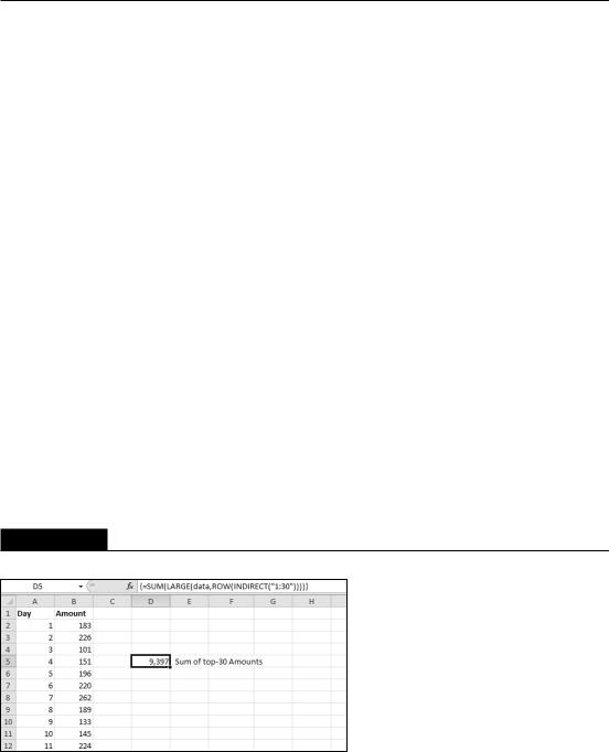
These formulas use an array constant comprised of the arguments for the LARGE or SMALL function. If the value of n for your top-n calculation is large, you may prefer to use the following variation. This formula returns the sum of the top 30 values in the Data range. You can, of course, substitute a different value for 30.

{=SUM(LARGE(Data,ROW(INDIRECT(“1:30”))))}

Figure 13.13 shows this array formula in use.

FIGURE 13.13

Using an array formula to calculate the sum of the 30 largest values in a range.

302