

up or down rather than wait?
4.3 Making assumptions
To make progress with our model building, we must make some assumptions; in fact, keeping the ‘building’ metaphor in mind, if the factors are the building blocks, the assumptions provide the cement with which to put the structure together. The ultimate success or failure of our model will very likely depend on whether we make an apt choice of assumptions and this is where the expertise of an experienced modeller becomes evident. Having said how important it is to make suitable assumptions, we have to go on to admit that experience counts here, more than in any of the stages involved in modelling, and it is unfortunately difficult to give general advice to beginners.
A variety of assumptions may be necessary, e.g. the following.
1.Assumptions about whether or not to include certain factors.
2.Assumptions about the relative sizes of terms or the relative magnitudes of the effects of various factors.
3.Assumptions about the forms of relationships between variables.
Generally speaking, and especially when developing a new model for the first time, we try to choose assumptions which keep the model as simple as possible. Always take care to write down your assumptions clearly so that you are aware of them yourself and that later on when explaining your model to others they will be able to see exactly what assumptions have been made. Look back at the examples in chapter 2 and make a list of the assumptions which were made in each example. Do you think that they are reasonable?
Try to note all the consequences of your assumptions. Wherever possible, test your assumptions against data (see chapter 8). Beware of implicit assumptions which you may make without realising that you have made them. In the previous section, we did not assume anything about friction in the pipes. By leaving out pipe friction from the model, we did in fact assume that friction was negligible.
For models involving mechanics (there are some examples in chapter 6), we are helped by the fact that there are well tried and tested assumptions and we can follow the example of previous modellers from the time of Newton.
Closely allied with assumptions are modelling decisions which we usually have to make, the most important of which are as follows.
1.What is the appropriate level of detail to include in our model? We always have to struggle towards a compromise between the complexity of the real problem and the need to produce a limited but useful model within the finite time and resources available to us.
2.Should we try an analytic model or a simulation model?
3.Should we model the variables as discrete or continuous?
4.Should we use a stochastic or a deterministic model?
While debating these questions, remember the purpose of your model and do not try to be too ambitious.
4.4 Types of behaviour
When variables affect each other, the way that one variable behaves when another is varied is most
conveniently expressed in terms of a graph with one variable plotted on the horizontal axis and the other on the vertical axis. We often think of the variable measured on the horizontal axis as the independent variable and the other as the dependent variable. In many problems the independent variable is time and we are looking at the time behaviour of our variables. Alternative ways of describing the relationship between two variables is by a mathematical formula or a table. In modelling, we often need to translate from one form to another. We can easily produce the graph corresponding to a particular formula but finding a mathematical formula corresponding to a graph or a table is not so easy and we look at ways of doing this in chapter 8.
In the case of input variables, we may have only a vague idea of how they behave, in which case we assume the simplest mathematical forms which give the right kind of behaviour as far as we can judge. Sometimes there
are some data to guide us and, if a substantial number of data are available, we can use the methods of chapter 8 to fit an appropriate mathematical form.
It is particularly useful to consider the following questions. (We shall assume that t is the independent variable and y is the dependent variable.)
1.What happens at large t ?
2.What happens at small t ?
3.Are there any values of t for which y has a local maximum or minimum?
4.Are there any values of t for which y = 0?
5.Are we interested in all values of t or only a certain range, say t > 0 or t 1 < t < t 2 for positive t 1 , t 2 ?
In the case of output variables, whether we present their behaviour in graphical, formula or tabular form depends partly on personal preference and partly on how complicated our model is.
The following is a collection of simple types of behaviour which are very commonly used in modelling. More complicated types can be built up by combining these simple forms together. The letters a, b and ω represent parameters taking real positive values and we assume that t starts at 0 and takes real positive values only. Note that, apart from the linear case, the mathematical expressions quoted are just the simplest forms showing that particular behaviour. Many other mathematical expressions with a similar behaviour exist.
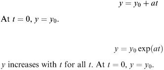
Linear (Figure 4.2)
Growing without limit (Figure 4.3)
Increasing to a limit (Figure 4.4)
Decaying to a limit (Figure 4.5)
Simple maximum (Figure 4.6)
Maximum followed by tailing off (Figure 4.7)
Oscillatory (Figure 4.8)
Decaying oscillations (Figure 4.9)
y = 0 at t = 0 and at t = n π/ω where the period is 2π/ω. The amplitude decreases with increasing t. The ratio of successive amplitudes is exp(−2 b π/ω).
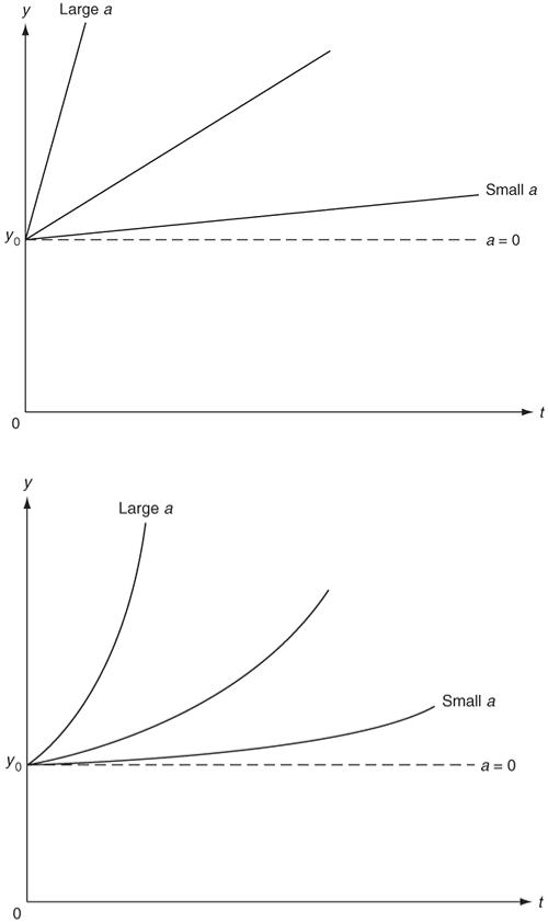
Figure 4.2
Figure 4.3
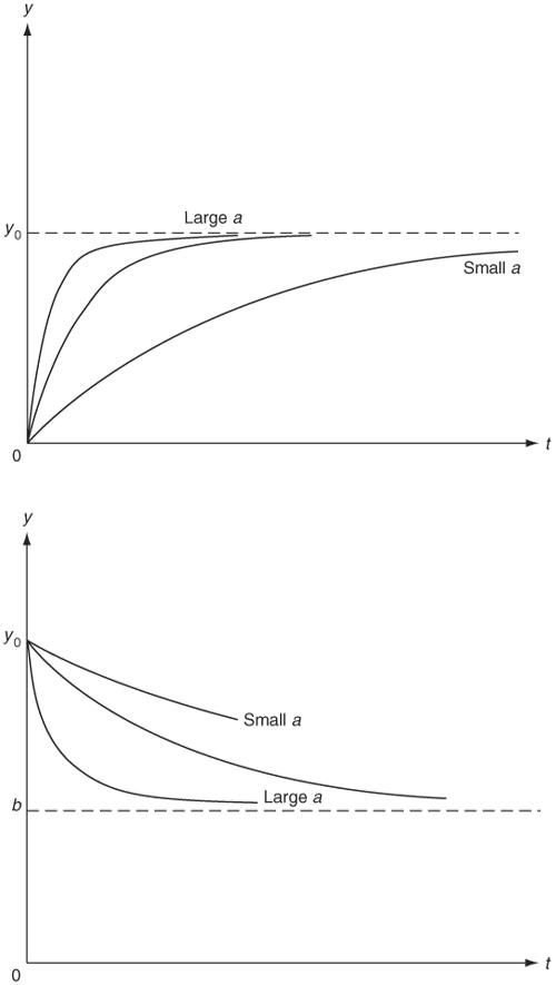
Figure 4.4
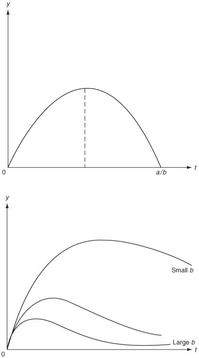
Figure 4.5
Figure 4.6
Figure 4.7
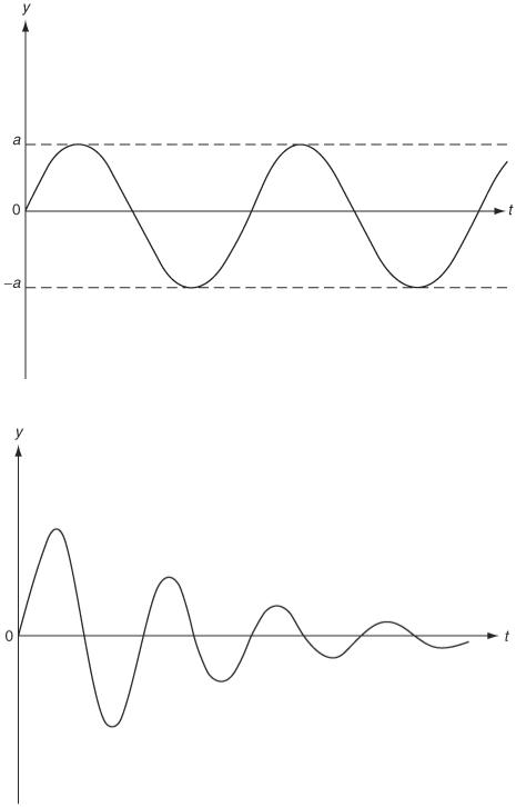
Figure 4.8
Figure 4.9
Example 4.2
A culture of bacteria is growing rapidly. If its size now is 100 organisms and the population doubles in size every 5 min, what expression could we use for the population size at time t ?
Solution
If we assume that y = y 0 exp( at ), then at t = 0 we have y = y 0 = 100. At t = 5, y = 200 = 100exp(5 a ). Therefore, a = 1/5 1n 2  0.139. So a possible model is y = 100exp(0.139 t ). Note that, as it stands,
this model implies that the population continues to grow without limit. In practice, limitations of space and/or food supply will prevent this and we need to restrict the domain of validity of our model to some finite interval of time.
Example 4.3
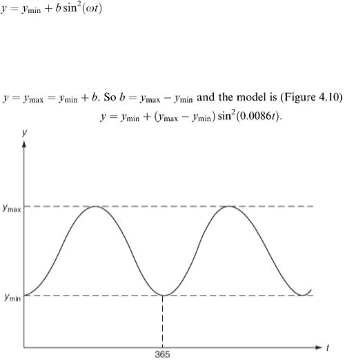
Suppose that we wish to model the daily average number of hours of sunshine at a particular location. If we start measuring from the winter minimum when the average number of hours of sunshine is y min and let t be the time in days from this point, then a suitable simple model might be
What values should we take for b and ω? Solution
The period of sin 2 (ω t )(which = [1 – cos2ω t ]) is π/ω = 365 days; so ω = π/365  0.0086. If y max is the value at the summer peak, this occurs when ω t = π/2, i.e. when
Figure 4.10
Example 4.4
In many situations, if the price of an article is increased, the number of articles bought decreases. A simple model for this kind of behaviour is y = y 0 − ap, where y is the number of articles sold when the price is p. What values should we take for y 0 and a ?
Solution
When the price is increased by one unit, a is the decrease in y. y 0 is the number theoretically sold when p = 0, i.e. when the articles are given away free! This is somewhat artificial and a better idea would be to take two points, i.e. to estimate the numbers that would be sold at two different prices p 1 and p 2 . Suppose that we estimate these to be y 1 and y 2 . Then y 1 = y 0 − ap 1 and y 2 = y 0 − ap 2 ;
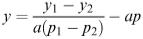
so y 2 = ( y 1 − y 2 )/ a ( p 1 − p 2 ) and the model is
An appropriate domain of validity for the model would be the interval p 1 < p < p 2 . The model could be used for p values outside this range but only at the user's risk.
Exercises
Which of the following expressions
1.are increasing for all x,
2.are very large for small x,
3.become very small at very large x and
4.are unbounded for large x ?
1.
2.1 − exp(− x )
3.x exp(− x )
4.5
4. 
5. 
6. 
7. 
8. 
4.6Do the following expressions increase or decrease
1.as a increases,
2.as b increases and