- •Preface
- •1.1 Introduction
- •1.2 Models and modelling
- •1.3 The learning process for mathematical modelling
- •Summary
- •Aims and objectives
- •2.1 Introduction
- •2.2 Examples
- •2.3 Further examples
- •Appendix 1
- •Appendix 2
- •Aims and objectives
- •3.1 Introduction
- •3.2 Definitions and terminology
- •3.3 Methodology and modelling flow chart
- •3.4 The methodology in practice
- •Background to the problem
- •Summary
- •Aims and objectives
- •4.1 Introduction
- •4.2 Listing factors
- •4.3 Making assumptions
- •4.4 Types of behaviour
- •4.5 Translating into mathematics
- •4.6 Choosing mathematical functions
- •Case 1
- •Case 2
- •Case 3
- •4.7 Relative sizes of terms
- •4.8 Units
- •4.9 Dimensions
- •4.10 Dimensional analysis
- •Summary
- •Aims and objectives
- •5.1 Introduction
- •5.2 First-order linear difference equations
- •5.3 Tending to a limit
- •5.4 More than one variable
- •5.5 Matrix models
- •5.6 Non-linear models and chaos
- •5.7 Using spreadsheets
- •Aims and objectives
- •6.1 Introduction
- •6.2 First order, one variable
- •6.3 Second order, one variable
- •6.4 Second order, two variables (uncoupled)
- •6.5 Simultaneous coupled differential equations
- •Summary
- •Aims and objectives
- •7.1 Introduction
- •7.2 Modelling random variables
- •7.3 Generating random numbers
- •7.4 Simulations
- •7.5 Using simulation models
- •7.6 Packages and simulation languages
- •Summary
- •Aims and objectives
- •8.1 Introduction
- •8.2 Data collection
- •8.3 Empirical models
- •8.4 Estimating parameters
- •8.5 Errors and accuracy
- •8.6 Testing models
- •Summary
- •Aims and objectives
- •9.1 Introduction
- •9.2 Driving speeds
- •Context
- •Problem statement
- •Formulate a mathematical model
- •Rewritten problem statement
- •Obtain the mathematical solution
- •9.3 Tax on cigarette smoking
- •Context
- •Problem statement
- •Formulate a mathematical model
- •Obtain the mathematical solution
- •9.4 Shopping trips
- •Context
- •Problem statement
- •Formulate a mathematical model
- •Obtain the mathematical solution
- •Interpret the mathematical solution
- •Using the model
- •9.5 Disk pressing
- •Context
- •Problem statement
- •Formulate a mathematical model
- •Obtain the mathematical solution
- •Interpret the mathematical solution
- •Further thoughts
- •9.6 Gutter
- •Context and problem statement
- •Formulate a mathematical model
- •Obtain the mathematical solution
- •9.7 Turf
- •Context
- •Problem statement
- •Formulate a mathematical model
- •Obtain the mathematical solution
- •Interpret the solution
- •9.8 Parachute jump
- •Context and problem statement
- •Formulate a mathematical model
- •Obtain the mathematical solution
- •9.9 On the buses
- •Context
- •Problem statement
- •Formulate a mathematical model
- •Obtain the mathematical solution
- •9.10 Further battles
- •Discrete deterministic model
- •Discrete stochastic model
- •Comparing the models
- •9.11 Snooker
- •Context
- •Problem statement
- •Formulate a mathematical model
- •Obtain the mathematical solution
- •Interpret the mathematical solution
- •9.12 Further models
- •Mileage
- •Heads or tails
- •Picture hanging
- •Motorway
- •Vehicle-merging delay at a junction
- •Family names
- •Estimating animal populations
- •Simulation of population growth
- •Needle crystals
- •Car parking
- •Overhead projector
- •Sheep farming
- •Aims and objectives
- •10.1 Introduction
- •10.2 Report writing
- •Preliminary
- •Main body
- •Appendices
- •Summary
- •General remarks
- •10.3 A specimen report
- •Contents
- •1 PRELIMINARY SECTIONS
- •1.1 Summary and conclusions
- •1.2 Glossary
- •2 MAIN SECTIONS
- •2.1 Problem statement
- •2.2 Assumptions
- •2.3 Individual testing
- •2.4 Single-stage procedure
- •2.5 Two-stage procedure
- •2.6 Results
- •2.7 Regular section procedures
- •2.8 Conclusions
- •3 APPENDICES
- •3.1 Possible extensions
- •3.2 Mathematical analysis
- •10.4 Presentation
- •Preparation
- •Giving the presentation
- •Bibliography
- •Solutions to Exercises
- •Chapter 2
- •Example 2.2 – Double wiper overlap problem
- •Chapter 4
- •Chapter 5
- •Chapter 6
- •Chapter 8
- •Index
i.e.
(9.7)
Obtain the mathematical solution
A units check is useful for equation (9.7). Referring back to chapter 4, we can see that both sides have dimension L/T. Note also that an initial state is required (as is the case for any differential equation). Equation (9.7) is a first-order equation and a suitable initial condition might be h (0) = 0, i.e. the gutter is dry and it starts to rain. There is a mathematical difficulty with this condition, however, in that equation (9.7) is ‘singular’ at h = 0, i.e. we cannot evaluate h ′(0) when h = 0 is substituted. This situation may be avoided by working with dt /d h instead, or taking h (0) = 1.0 cm, for example. What would be the effect of trying other starting values?
Some data have been given above for this model, but a full list is now convenient: a = 0.075 m; b = 6.0 m; d = 12.0 m; g = 9.81 m s −2 ; A = 0.0025 πm 2 ; α = 30°. Substituting these values into equation (9.7) gives
(9.8)
Solving the differential equation (9.8) will give us h(t), the height of water in the gutter at any time. Our problem is now in the form, given the rainfall rate r(t), find the depth h(t).
Two possible expressions for the rainfall rate r(t) are as follows:
or
The first model is the equivalent of steady persistent rain which sets in over a long period. Either the gutter overflows as it cannot cope, or a steady state will arise where the depth of water in the gutter h(t) settles to a constant value of less
than 0.075 m. From equation (9.8) the steady state can be mathematically predicted by examining what happens if h ′ ( t ) = 0, which applies when there is a steady state:
For example, r = 0.025 cm s −1 a steady-state situation occurs at h 5 cm, as can be seen from Table 9.11 and from the graph (Figure 9.12).
For the second model (illustrated in Figure 9.13) the rain profile represents a short heavy burst which rises to a peak at 20 s and then decreases to zero at 40 s. Thus we would expect the gutter to fill up rapidly before the level falls off. This is the behaviour predicted by the model when equation (9.8) is rewritten as
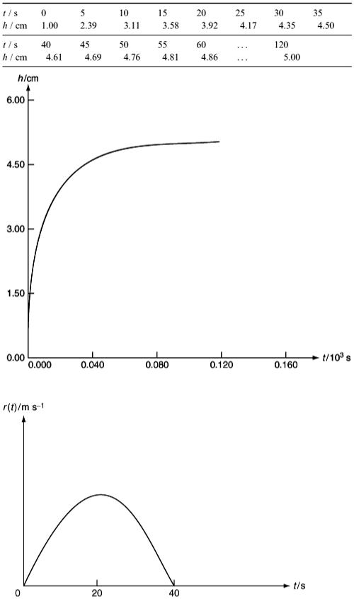
Table 9.11
Figure 9.12
Figure 9.13