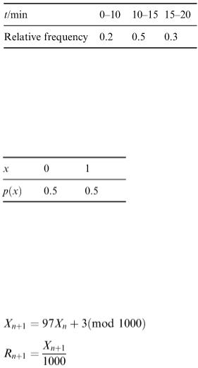
min. He records the time t on a number of occasions and tabulates the data as follows.

This is an example of a frequency table (or, when plotted graphically, a histogram) for a continuous random variable.

7.3 Generating random numbers

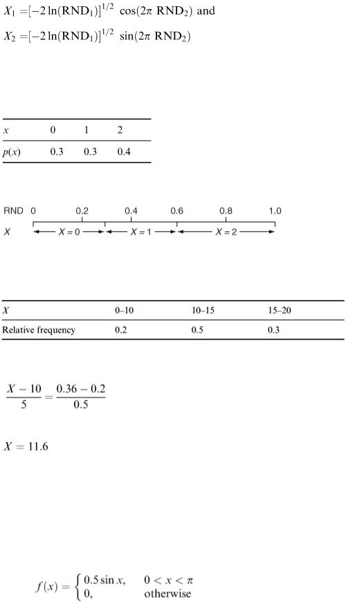
The toss of a fair coin produces a random outcome which can be used as an observation of the discrete random variable X whose probability function is the following.

If we needed to simulate a value or a set of values of this random variable, we could do it by tossing the coin and recording the results. This is rather limiting, however, and for random variables with other distributions we use computer-generated pseudo-random numbers. These are produced in a sequence based on a formula. The numbers obtained do not have any obvious pattern and, when suitably scaled, it is found that their distribution corresponds very closely to the uniform distribution on the interval [0,1].

An example of such a formula is

An arbitrary starting value (‘seed’) is taken—for example X 0 = 71; then, to get X 1 , we substitute for X 0 in the formula, which gives 6890. Next we count any multiples of 1000 as being equivalent to zero, which gives 890. We then divide by 1000 to give R 1 = 0.890. Substituting X 1 = 890 gives R 2 = 0.333… and so on for as long as we like. (Eventually we shall get back to 71 and repeat the cycle but only after a very long time.)

In many high-level programming languages and on pocket calculators a standard function usually represented by some name such as RND produces a pseudo-random number of this kind. From now on, we shall use RND to stand for a generated random value from the uniform continuous distribution on [0, 1].

We can build other random variables from this. For example X = a + ( b − a ) RND gives a random variable whose distribution is the continuous uniform distribution on the interval [ a, b ].

If we want to produce values for the exponential distribution with parameter λ, we use X = −(1/λ) In (RND) or, more conveniently, X = − m In (RND), where m is the mean.

Values for the Normal distribution with a mean of 0 and a standard deviation of 1 can be produced by taking two RND values and then using the formulae

to give two values of X. If values from the Normal (μ, σ 2 ) distribution are required, then use X = σ X 1 + μ or σ X 2 + μ.

To obtain values for discrete random variables, divide the [0, 1] range into appropriate parts. For example, suppose a discrete random variable has the following probability function.

Take an RND value; then, if 0 < RND < 0.3, this means X = 0, if 0.3 < RND < 0.6, this means X = 1, and, if RND > 0.6, this means X = 2.

This ensures that the values 0, 1 and 2 come up statistically with the right frequencies.

We use the same idea for a continuous random variable tabulated into classes except that we take the generated value of the random variable to be the class midpoint.

An RND value of 0.36 would be translated into X = 12.5. A refinement would be to use linear interpolation rather than just to take the midpoint, i.e.

giving

To simulate a theoretical distribution for a continuous random variable with known pdf, there are two main methods available.

1.The inverse cumulative distribution function method If the pdf of a random variable is f ( x ), the cumulative distribution function is 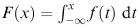and if regarded as a random variable, F is uniformly distributed on [0, 1]. A value of RND is taken from the uniform [0, 1] distribution; then the equation RND = F ( x ) is solved to find the corresponding value of x (= F −1 (RND)). For example, suppose that

The graph is shown in Figure 7.4

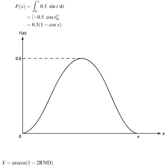
The cumulative distribution function is

Figure 7.4

Inverting RND = 0.5(1 − cos X ) gives

This is the formula we need for generating X values for this distribution.

The rejection method For this, we need two RND values to generate one X value. Suppose that f(x) = 0 except on the interval [a, b] and that the maximum value of f(x) is c (Figure 7.5). To generate an X value, we go through the following steps. Generate RND1 and RND2 from the uniform [0, 1] distribution. Use RND1 to calculate x = a + (b − a) RND1. Calculate f(x). Use RND2 to calculate y = cRND2. If y < f(x), then accept x; otherwise reject x and return to step (a).

For the above example, we would use a = 0, b = π and c = 0.5.

You can see that the RND function provides us with the raw material that we need to generate sample values of random variables. This is called ‘simulation’ and it breathes life into our probabilistic models. Note that in this chapter we are using the term ‘simulation’ as short-hand for ‘stochastic simulation’ (see section 3.2 for a wider discussion on simulation).

Figure 7.5

7.4 Simulations

What we mean here by a simulation is a probabilistic model set in motion by a stream of random numbers. As a simple example, consider the following problem.

Example 7.1

A train leaves station A at a time which is about 1.00 pm but distributed as follows.

The train's next stop is at B where you are hoping to catch it. The train's journey time from A to B is variable with a mean value of 30 min and a standard deviation of 2 min. Your time of arrival at B is distributed as follows.

What is the probability that you catch the train? An equivalent way of posing the question is on what percentage of occasions under these identical conditions will you catch the train? It is this second (relative frequency) interpretation which we use to obtain an answer by simulation. We need random numbers; so we shall use those given by the formula in section 7.3, which are 0.890, 0.333, 0.304, 0.491, 0.630,…. What we need to simulate are the following.

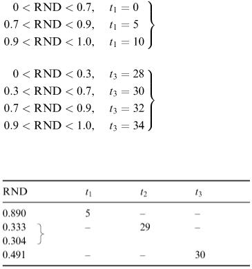
1.The departure time t 1 of the train.

2.The journey time t 2 of the train.

3.Your arrival time t 3 at the station.

We are interested in whether t 3 < t 1 + t 2 .

To run the simulation, we simply need to produce values for t 1 , t 2 and t 3 and to test the condition. It is not obvious how to get a value for t 2 . We do not know the distribution; so we shall have to assume a model. Let us take the normal distribution with a mean of 30 min and a standard deviation of 2 min. Note that we are treating t 1 and t 3 as discrete and t 2 as continuous. This is only because of the way that our data were presented.

Using a minute as the time unit and counting from t = 0 at 1.00 pm our model is made up as follows:

t 2 = 2 X + 30

where X = [−2ln(RND 1 )] ½ cos(2πRND 2 ). The calculation gives the following table.

So, on this occasion, you arrive 4 min before the train comes in. Note that we must not use the same RND value for more than one purpose. This would lead to false correlations between variables in our model.

The conclusion from this single run of the model is that you caught the train, but obviously this does not answer the original question. We need to do several runs and to record the percentage of runs on which we catch the train. The answer that we get can only be regarded as an approximation. To find the exact answer by this method, we would have to carry out a theoretically infinite number of runs. This is a feature of all simulation models. We must carry out many runs and calculate averages from our results. Clearly, it will be a great help if we implement our model in the form of a computer program.

The above example is rather trivial and far from typical of the kind of model for which simulation is usually used. In practice, we normally refer to the set of circumstances which we are trying to model as a ‘system’. We shall take a simple model of a hairdresser's shop as an example of a system.

Example 7.2

Customers arrive at a hairdresser's shop at random times. There are two assistants, A and B. 60% of customers require a cut, which takes 5 min; the other 40% require a shampoo and cut, which takes 8 min.

Generally speaking, the basic elements needed for carrying out any simulation are as follows.

1.A set of state variables whose values completely describe the system at any time.

2.A procedure for calculating new values of the state variables at time t + 1 from those at time t. In our example there are three state variables.

1.The number of customers waiting (discrete non-negative integer).

2.Whether or not A is busy (yes or no).

3.Whether or not B is busy (yes or no).

A run of the simulation consists of a series of calculations starting with the values of the state variables at t = 0 and ending at some time t = END. An event is a point in time when a state variable changes its value. In our example the events are as follows.

1.An arrival.

2.Start of service by A.

3.End of service by A.

4.Start of service by B.

5.End of service by B.

An entity is a discrete item which either is a permanent part of the system or enters and leaves, e.g. a customer, a lorry or an order. Here the entities are the customers and the two assistants.

There are two types of procedure for studying a simulation model.

1.Time slicing where we examine the state variables and the whereabouts of the entities at time slices (usually equally spaced). At each time slice the state variables may or may not have changed.

2.Event sequencing where we examine the system at each event, regardless of the time between events.

These two approaches are sometimes referred to as ‘time-driven’ and ‘event-driven’ models. Generally, we use time-driven models for continuous deterministic systems and event-driven models for probabilistic discrete systems, but this is not always the case and for this particular example we shall use both types.

For the time-slicing model, we must decide how large to make the time slices and for simplicity we shall take 1 min. The description of the problem did not contain any information about the rate of arrival of customers. Suppose that in any minute the probability that a customer arrives is 0.5. There are actually two kinds of customer, depending on whether they have come for a cut or for a shampoo and cut. We can make up a crude and simple model by taking the average service time 0.6 × 5 + 0.4 × 8 = 6.2 min and taking this to apply to all customers.

A coin will do as a random-number generator, where T is tails and H heads. Suppose that a sequence of tosses gives THTTHTTTHHT…. Taking T to indicate an arrival and taking the initial state to be no customers, we run through the first 10 min as follows.

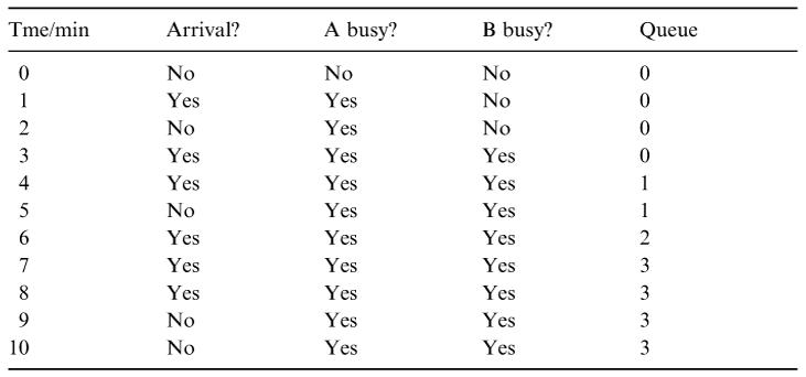
At this point, we shall stop to ask what we hope to get out of it. The usual things of interest are the average queue length, the maximum queue length, the average waiting time of customers, and the percentage busy times of the two assistants. We shall look at how to calculate these results in section 7.5. The point of creating the model is, of course, not just to try to mimic the real system but to obtain answers to questions. These will usually be questions about the effects of making changes such as employing an extra assistant, or altering the service time.

In our simple model, we have made a number of assumptions as well as gross simplifications.

1.We assumed (for our own convenience) that the probability of an arrival in any minute is 0.5. If we had data indicating that a more accurate figure would be 0.3, we could no longer use the coin. We would use the RND function, taking RND > 0.3 to mean that a customer arrives.

2.

We implicitly assumed that more than one customer would never arrive in the same minute. If this had been observed to happen, it would mean that our choice of 1 min as the time slice was not good; a smaller time would be better.

We assumed that, if both assistants were free, a customer would make a random choice between them. If necessary, we could build in a preference into our model. We assumed a ‘queue discipline’ of ‘first in, first out’ (FIFO). Some customers might have prior bookings and would get priority. In practice a customer might, on arriving and finding a long queue, decide not to stay. A customer who had been waiting a long time might also get tired of waiting and leave without being served. One of the assistants might take a short break. We could include all these possibilities in the model.

An event-sequencing model requires more work but enables us to get closer to the real situation. We use the term activity to refer to the time between two events. In our problem the activities are as follows.

1.The queueing time.

2.The service time by A.

3.The service time by B.

The duration of an activity may be constant or random. If random, then we need a distribution to model it. We also need to specify how many entities can use the activity in parallel. In our example there can be many customers waiting simultaneously but an assistant can only serve one at a time. Many systems can be regarded as consisting of entities passing through a number of activities. The paths taken by the entities can be shown in a flow diagram. If more than one entity can be engaged on an activity in parallel, we must show this in our flow diagram, and whether or not there is an upper limit.

An attribute is a property of an individual entity, e.g. the size of an order, or whether a lorry is full or empty. The attribute could be constant or could change during the simulation and there could be a number of attributes attached to each entity. In our example each customer has only one attribute – the type of service required.

It may be useful to think of a queue as a special kind of activity. The most obvious feature is that there will often be many entities engaged in this activity at the same time. There also has to be a queue discipline such as ‘last in, first out’ (LIFO) or FIFO and, when there is more than one queue leading to the same activity, we need rules to state which queue has priority. We may also need priority rules within a single queue. These may be based on the attributes of the entities, e.g. ‘empty lorries have priority’. Queues are different from other activities in that the length of time that an entity stays in a queue depends on

factors such as the number of other entities in the queue, priorities and rules. We cannot just sample the queuing time from a distribution.

Another special activity required is the generating activity for generating arrival events. This activity represents the inter-arrival time and we often use the exponential distribution as a model.

To carry out the simulation, we generally have the following options.

1.Work it through by hand.

2.Use a specially written computer program.

3.Use a computer package or simulation language.

Option 1 is obviously the most tedious and least efficient but it has the merit of helping us to sort out our ideas clearly. It is often a good idea at least to start a hand simulation until we are confident that we have modelled all the necessary details correctly. We can then turn to option 2 or option 3.

The standard procedure for carrying out a hand simulation involves the following steps.

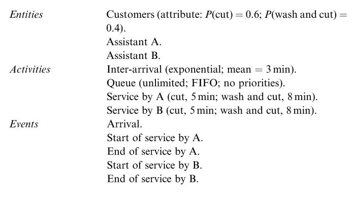
1.Make a list of the entities (and attributes if any), state variables, activities and queues. For each activity, write down starting conditions (if any), method of determining duration, and the maximum allowed number of entities in parallel. For each queue, state the queue discipline and any other operating rules. Write down the starting conditions and the end time (or ending condition) for the simulation.

For the hairdresser's example, let us assume that the inter-arrival time has the exponential distribution with a mean of 3 min. We can then simulate the time between arrivals by –3 In(RND) (min). Let us work through the simulation as far as the arrival of the tenth customer. We list the complete problem as follows.

1.Draw a flow diagram (Figure 7.6) showing the events and activities. This shows the paths that we have to trace out as we follow through the simulation and it can be useful in constructing a computer program. Remember that events are points in time, and activities are things that take time.

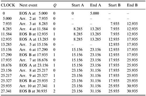
2.Draw up a table (‘trace table’) which will enable you to step through the simulation from event to event. This should include the time since the start of the simulation (‘CLOCK’), the next event and the state variables on each line.

3.Produce as many RND values as you need. You may use these as you wish, provided that you do not use the same value twice. Either produce them as and when they are needed or produce them at the beginning of the simulation and convert them into the required information. For our hairdresser's shop we need a total of 19 RND values, nine of them for the inter-arrival times and one for each customer to find out whether they have come for a cut (RND < 0.6) or a wash and cut (RND > 0.6).

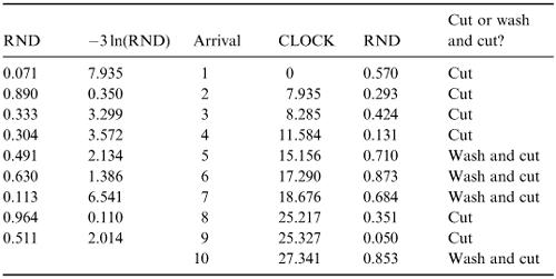
We have used the random-number sequence from section 7.3 and converted the first nine (from 0.071 to 0.511) into arrival times by the formula –3ln (RND). The next 10 (from 0.570 to 0.853) have been used to decide the type of service required for each customer.

Note that we have started the CLOCK at the time of the first arrival and accumulated the interarrival times to get the CLOCK times for subsequent arrivals. We have kept accuracy to three decimal places, which probably was not necessary.

Figure 7.6

Fill in the trace table, taking care to identify the next event correctly at each step. We have used the abbreviation EOS for ‘end of service’ and Arr. 2 for ‘Arrival number 2’, etc.

Note that we have assumed that as soon as an assistant has finished serving one customer he or she instantly takes another one (if there is one) from the queue. Note also that the queue does not include customers being served. Many mathematical modellers do include the customer being served as being still in the queue. Watch out for this and make sure that you have explained your method clearly.

It seems rather unrealistic to assume constant service times of 5 and 8 min. If we wanted to allow variable service times, how would we do it? The choices are either to assume some models for the distributions, such as a uniform distribution of between 4.5 and 5.5 min for a hair cut or, if data are available, to take sample values using the relative frequencies as we did in section 7.3. We could obviously assume different distributions for the two assistants instead of assuming that they are identical as we have done.

Exercises

7.1Obtain an answer for Example 7.1 (the probability of catching the train). Run the hairdresser's shop model using the following information.

1.When the shop opens, there are no customers waiting.

2.The inter-arrival time of customers has the exponential distribution with a mean of 3 min.

3.60% of customers require a cut and 40% require a shampoo and cut.

7.24. Assistant A's service time is exponentially distributed with a mean of 5 min for cutting and a mean of 8 min for washing and cutting.

5.Assistant B's service time is exponentially distributed with a mean of 4.5 min for cutting and a mean of 7 min for washing and cutting.

6.Customers finding a queue of six people or more when they arrive will not stay.

7.Both assistants will take a 1 min rest after serving five customers without a break.

Run the model until 30 customers have passed through the system. Calculate the average waiting time, the average queue length and the number of customers who turned away. Also calculate the percentage busy time for both assistants. How would these figures change if

1.assistant A's mean service times could be reduced to those of B?

2.the mean inter-arrival time became 2 min or less?