predict for it?

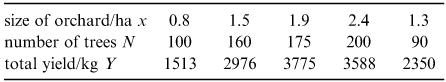
The following table gives the yield of fruit from each of five orchards of different sizes and also the number of fruit trees in the orchard. Too many trees reduces the amount of fruit on each tree so the question is: given an orchard of size x (ha), how many trees ( N ) of this kind should be planted so as to get the maximum possible yield?

8.12

Decide what are the most relevant variables to plot before trying to fit a model.

Explain why plotting Y against N would not be a good idea.

8.5 Errors and accuracy

Our data very often come from experimental observations and measurements made with imperfect instruments; so we cannot hope to avoid errors. The errors in the data are of course in addition to the errors that we make during the modelling. We can list the various sources as follows.

1.Errors due to our modelling assumptions.

2.Errors due to using an approximate method of solution.

3.Errors due to carrying out inexact arithmetic (rounding errors).

4.Errors in the data.

With all these errors about, it is clear that our modelling predictions cannot be 100% reliable. We have a duty, however, to try to estimate what the maximum error in our prediction is likely to be. In other words, we ought to try to produce a statement of the form ‘we predict X with a possible maximum error of Y (or Z %)’.

Errors can be described in more than one way. We define absolute error to be the difference between a true value and an approximate value. For example, if we use 22/7 as an approximation for π the absolute error is π − 22/7 −0.0012645. An absolute error of 0.1 with respect to a measurement of magnitude 1000 represents greater accuracy than an absolute error of

0.1 in a measurement of magnitude 10. To allow for this distinction, we use relative error, defined by relative error = (absolute error)/measurement. It is often expressed as a percentage. For example, the relative error in 22/7 when used as an approximation for π is 0.0012645/π 0.0004025 or about 0.04%.

Let us now look at the above-listed sources of error.

1.It is almost impossible to be sure about the effects of errors due to our modelling assumptions because we do not normally know the correct value of the answer that we are trying to estimate. We can do a certain amount of investigation by varying the assumptions and noting the effect on the answer.

2.We often use approximate (numerical) methods, either because mathematical solutions are

impossible to obtain or just because it is quicker to use a computer. These numerical methods involve errors (truncation errors) depending partly on the data and partly on the type of method used. Sometimes, we use shorter or easier mathematical expressions in place of others such as when we replace sin x by x and cos x by 1 when x is small. This also involves us in truncation errors.

3.Any numerical work that we carry out using an electronic aid such as a calculator or computer inevitably involves rounding errors because of finite storage capacities. These rounding errors can accumulate to an appreciable amount if we do a large amount of computation.

4.Ideally, an estimate of the maximum error in the data should be available.

The way in which all these errors combine together is complicated. As modellers, we should try to identify the most serious source of error and also to estimate the worst possible error in our final prediction.

Example 8.7

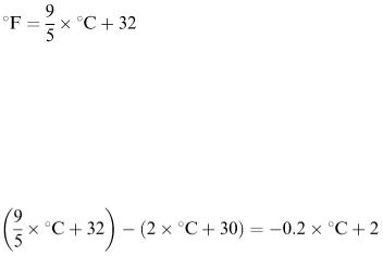
In chapter 4, we mentioned the formula for translating from temperatures measured in degrees Celsius to the equivalent temperatures in degrees Fahrenheit:

A simpler model would be °F = 2 × °C + 30 and this is simple enough for us to do the calculation in our heads. For example 20°C becomes 70°F according to the simple model, while the exact formula gives 68°F. How accurate is this simple formula over the range of air temperatures normally experienced in this country?

Solution

The absolute error is

For the range −5 < °C < 25 the error varies from 3 to −3 with a maximum percentage error of about 22% at °C = −5. If we restrict the model to positive temperatures, the error varies from about 5% at 0°C to about 10% at 25°C.

Remember that there is no practical advantage in having a very accurate model if an approximate model is easier and quicker to use and gives answers that are sufficiently accurate for practical use.

Exercises

The function sinh x is defined by sinh x = [exp x – exp(− x )]/2. As x increases, exp x increases

8.13while exp (− x ) decreases; so we can expect that, for sufficiently large x, sinh x can be approximated by (exp x )/2. How large does x have to be for this to be accurate to less than 5%?

When the Earth is modelled as a sphere (of diameter 12.72 × 10 3 km), it is obvious that, if the

8.14walls of a tall building are vertical, they cannot be parallel. Suppose that a tower block is 400 m tall and that the ground floor has an area of 2500 m 2 . How much extra area is there on the top floor?

8.15A railway line is exactly 1 mile long and one night a vandal cuts the line in the middle and inserts

an extra foot of metal. The line is constrained at its two ends; so it is now forced to bend into an arc of a circle. How high above the ground is it at the midpoint?

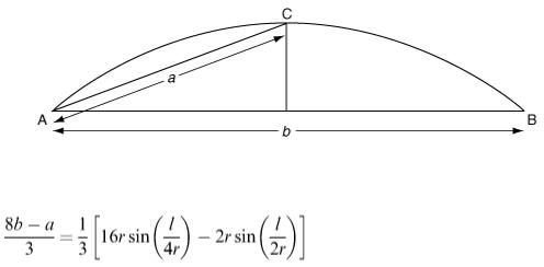
In Figure 8.15, C is the midpoint of an arc AB of a circle. An estimate of the length of the arc is given by (8 b − a)/3, where a and b are the lengths of AC and AB, respectively. How accurate is this estimate? You may like to show that, if l is the required length of arc and r is the radius of the circle, then

8.16

Figure 8.15

The approximation l (8 b − a )/3 can be obtained from this by using series approximations for the sin terms.

8.6 Testing models

The success of a model can be measured in terms of how well its predictions compare with what is actually observed in the real world. In the previous two sections, we have discussed the procedure of making our model fit available data. The real test of a model comes when we use it to make a prediction for data which we do not have.

By ‘testing’ a model, we do not mean finding out whether it is ‘correct’. In a sense, it is bound to be ‘wrong’ because it is only a model and has been derived by making simplifying assumptions. When we test a model, what we are trying to find out is whether it gives predictions which are sufficiently accurate to be useful.

In particular, does it adequately fulfil the purpose for which it was designed? Remember always that a model should give useful predictions that can be directly applied to the real world. Suppose that you have worked out a clever model for the game of snooker which can produce a prediction such as ‘to pot the black ball into the top right-hand pocket, the cue ball should be given an initial velocity of 1.5 m s −1 at an angle of 52° to the top cushion’. This could be, scientifically speaking, a very accurate prediction but of what practical use would it be to the player who is about to pick up his cue and play the shot? A good model should provide direct practical advice.

In general we expect our models to do more than to predict a single answer. We should be able to derive both qualitative and quantitative statements from our model, e.g. ‘ y increases as x increases’ or ‘ y is proportional to x ’.

The simplest way to test these statements (assuming some data are available) is to draw graphs. The

simple model of Example 8.4 predicts that people's weights will be proportional to the cubes of their heights. We can use the data to test this prediction but instead of plotting weight against height, which our model predicts will be a cubic curve, a better idea is to plot weight against (height) 3 . According to the model, this graph should be a straight line and departure from a straight line is easier to assess. The plot of ln H against ln W, of course, serves the same purpose.

Not suprisingly (Figure 8.7) the points do not lie exactly on a straight line. We have to decide whether they are close enough for the model to be useful.

Note that we do not need to know the value of the parameter. We are testing to see whether the points lie on a straight line and not on some particular line.

When testing any model, try to derive a relationship which your model predicts will be a straight line; then plot the corresponding data on graph paper. Ideally, you should decide what kind of test you are going to do and then collect the relevant data.

When the testing (or, as it is often called, the ‘validation’ or ‘verification’) of your model has proved disappointing, your task as a modeller is to decide whether to go back to the formulation stage and to improve the model or to scrap it altogether and to start again. Hopefully, the less drastic course of action is chosen. How do you improve your model?

Look at the list of factors again. Have you omitted one which ought to have been included? Have you lumped together some factors which should be considered separately? Look at your assumptions again. Can they be relaxed or made more general? For example, where you have assumed a linear relationship, perhaps a non-linear one is more appropriate?

If you find that your model's predictions are sufficiently accurate but not perfect, try to assess the accuracy. As we saw in section 8.5, it is very important to give a bound (i.e. an upper limit) on the possible error. For example, the simple height–weight model W = 12.54 H 3 gave predictions which were within 47% of the correct values (the worst error).

If you have a reasonable number of data, calculate the standard deviation of the errors in your model's predictions so that you can give an approximate confidence interval for future predictions. Also remember to allow for the sensitivity of your predictions to changes in the parameter values and/or changes in the modelling assumptions. Make small changes to your model and find whether or not these give rise to large changes in the model's predictions.

Example 8.8

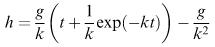
A stone is dropped down a vertical shaft in order to estimate the depth of the shaft by listening for the noise as the stone strikes the bottom. A student develops the following model relating time t and height h:

by assuming that the force on the stone due to air resistance is directly proportional to the speed of the stone, k being the proportionality constant.

If air resistance is neglected, the appropriate model is h = 0.5 gt 2 (motion under constant acceleration g ). This should agree with the student's model in the case k = 0 and we ought to check this. However, we cannot put k = 0 directly into the model (division by zero). Instead, if we expand the exponential term using Taylor's series

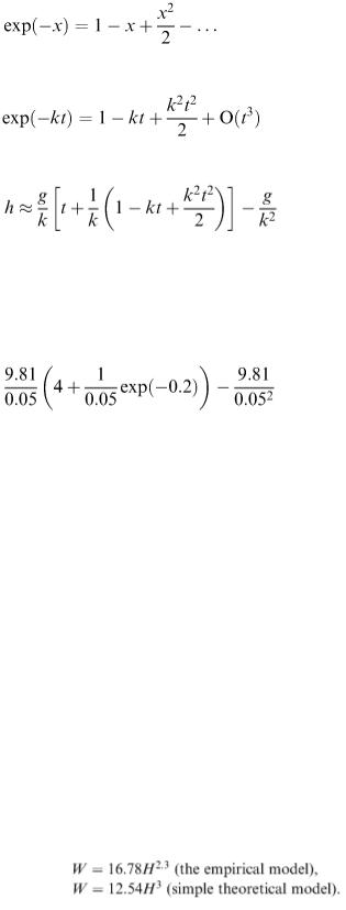
we obtain

and

which gives h = 0.5 gt 2 when k = 0.

In order to use the model to calculate h from t, we need the value of k. The student has been told that the appropriate value of k to use is 0.05s −1 . Is the model dimensionally correct?

For a particular shaft the noise is heard after 4s. From the model, we calculate h to be

which is about 73.50m. We now have an estimate of h but what if the ‘correct’ value of k is actually not 0.05; how much does it matter? If we change k by 10% and substitute 0.045, we get h 73.98 m; so a 10% uncertainty in k leads to less than 1% error in h and the model is not unduly sensitive to the value of k.

If the student had neglected air resistance in his or her model would the estimate of h have been very inaccurate? The simple model gives h = 0.5 × 9.81 × (4) 2 78.48 m. So we have an absolute error of about 5 m or a relative error of about 7%. We conclude that the inclusion of the air resistance has a significant effect.

Another assumption that has been made in this model is that the instant at which the stone hits the bottom and the instant that the noise is heard are the same, but we know that the speed of sound is finite (about 330 m s −1 ). Does this matter?

The correction to the value of t is the time that it takes for the sound to travel up, which is h /330 73.5/330 0.223s. Substituting t = 4 − 0.223 = 3.777 in the model gives h 65.77m. We conclude that allowing for the finite speed of sound, which the student completely forgot about, is even more important than allowing for the air resistance.

Exercises

8.17In sections 8.3 and 8.4, we derived the following two models for predicting weight from height for humans:

Which model gives the best fit to the data in Table 8.1?