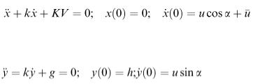
Equations of motion are horizontally:

6.10 vertically:

where V is the wind speed, ū the run-up speed and u the throw speed. Conditions for the ball to enter the basket:

6.11

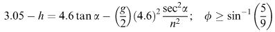
where Π is the angle of path with the horizontal on entry, u the initial throw speed and angle α, and h the height of the thrower.

6.13Approximately 53 h.

6.14d x /d t = − ay + R 1 , d y /d t = − bx + R 2 .

6.15d X /d t = aXF − bX, d Y /d t = c YF − d Y, d F /d t = − eX − fY.

Chapter 8

8.7T = 47.07 w 0.671 , 198 min.

8.8k 1.5.

8.989 − 20ln x

(a)T 2 = kR 3 . Confirm from logarithmic plot.

(b)R = 14.96(4 + 3 × 2 n −2 ) where n = 2, 3, …, 8 (the Titus–Bode law).

8.13x > 1.472.

8.140.314 m 2 .

8.15Approximately 50 ft.

8.17Using the least-squares criterion the second model is more accurate.

8.18(a) Y = 2.49 t, S 5.34 (b) Y = 0.97 t 2 , S 0.05

(c) Y = 0.44 exp( t ), S 0.41.

Model (b) has the smallest sum of squared errors, S.