

CHAPTER 6
Using Differential Equations
Aims and objectives
In this chapter we discuss models in which variables are represented as continuous functions of continuous time t. Assumptions have to be made about the rates of change of these variables and the resulting models involve differential equations.
6.1 Introduction
As mentioned in chapter 1, models are created with a particular purpose in mind and in many cases this purpose is to make predictions. These predictions may take the form of answers to such questions as ‘What happens to this variable if we increase (or decrease) that other variable?’ A successful model will have provided us with relationships between relevant variables from which we can obtain the necessary answers and, if it is a truly successful model, these predictions will be found to be verified when the data become available.
Very many models involve time as one of the variables and a very common question to ask in these cases is ‘What happens to all the other variables as time progresses?’ For these models we therefore need to consider rates of change of variables with time and it is a very likely consequence that our mathematical equations will contain derivatives. Such differential equations can be any of a wide variety of types, many of which cannot be solved analytically although approximate solutions can be obtained by numerical methods.
In any particular model, we arrive at a differential equation by considering the changes that occur in our variables over a finite but small time interval t. Dividing by t gives us finite rates of change and, letting t shrink to zero and taking limits, we obtain differential equations.
Such equations can be very difficult to solve exactly but there is no need to despair if the route to an exact solution appears closed. Much useful information about the behaviour of the solution can be gleaned from a differential equation without solving it. We can gain useful qualitative information by looking at such things as the magnitude and sign of the derivative for various values of the dependent and/or independent variables and, in particular, looking for values, if any, which make the derivative equal to zero. Good approximate solutions can be obtained by numerical methods and these can be just as useful as the exact analytic solutions.
Differential equations can be classified in many ways, the most fundamental being the order of the highest derivative occurring in the equation. In section 6.2, we use a first-order differential equation to model population growth, while in section 6.3, problems in mechanics are solved using a second-order equation. When our model involves several differential equations, they may be ‘uncoupled’, in which case each differential equation involves only one of the dependent variables, e.g.
Alternatively, they may be coupled, e.g.
Note that the independent variable t may also appear anywhere on the right-hand side of any of these equations.
In section 6.4, we have a model involving uncoupled equations, and in section 6.5, our examples involve coupled equations.
6.2 First order, one variable
Example 6.1
A model for population growth
If we want to create a model for predicting population growth, the variable in which we are interested is the size of the population at any time. This is the total number of living individuals in the population, ignoring the fact that they are of different ages, some are male, some are female, and so on. This total number is obviously a discrete variable but it makes the modelling easier if we pretend that it is a continuous variable P(t). This will not be a serious error when P(t) is large because a graph with very small discrete steps will be indistinguishable from a smooth curve.
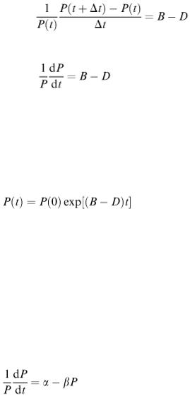
The purpose of our model will be to predict the future population, i.e. to give P(t) as a function of t. The most obvious reasons for a population to change are that individuals are born and some die but there could also be movement into and out of the area in which our population lives. So a simple model for the change in P(t) during a short period of time t is
For simplicity, we shall forget immigration and emigration. Clearly the number of births and deaths will depend on the following.
1. The size of the interval t.
2. The size of the population at the beginning of the time interval.
The simplest assumptions to make are that a strict proportionality applies in both cases; we then have
and
where B and D are constants. Our model is now
(6.1)
From this point we can develop our model in one of two different directions.
1. We could decide to use a finite time unit, say t = 1 year. Our variable P(t) would then be discrete, being defined only at intervals of one year. Equation (6.1) is a difference equation relating successive P values in the sequence P 1 , P 2 , P 3 ,…, where P n = P(n). We could write
the equation as P n +1 = ( B − D + 1) P n and the parameters B and D are the annual percentage birth rates and death rates respectively. To calculate the values P 1 , P 2 ,…, we need the value of P 0 , the population size at time t = 0. Difference equations are discussed in chapter 5, our subject in this chapter is differential equations.
2.The alternative is to regard the population as a continuous variable P(t) as we mentioned earlier. To proceed with our model, we first rewrite equation (6.1) as
Letting t → 0, this becomes
The expression on the left-hand side can be called the ‘proportionate growth rate’. Note that it does not have quite the same interpretation as in the discrete case because we are not tied to a particular time step here. If we use a small enough time step, however, both discrete and continuous models should agree and, if B − D is truly constant, equal to 0.04 say, this
would approximately correspond to a net growth rate (births minus deaths) of 4% per time unit. The solution of the differential equation is
where P (0) is the size of the population at time t = 0. This is a very simple model and predicts exponential growth without limit if B > D or exponential decay to zero if B < D.
In practice, of course, we do not see populations growing exponentially without limit. The growth may follow the exponential model for some time but eventually limitations of available space or food will tend to force the population level to ‘flatten out’. We can interpret this as the effect of overcrowding and/or food shortage, causing the birth rate to fall and the death rate to rise.
We can attempt to take these factors into account by allowing the proportionate growth rate (1/ P ) d P /d t to be a function of P rather than a constant. What function of P should we take? Obviously we need one that decreases with increasing P. The simplest model satisfying this requirement is a linear function, i.e.
where α and β are positive constants.
Before trying to solve this differential equation, we can work out some of its implications. If the population level reaches the value α/β, then the right-hand side will be zero, which means that d P /d t will be zero so that P will stop changing with time. Also, when we start with a population size P (0) at time t = 0, then the right-hand side of the differential equation is α − β P (0). If this is positive, then d P /d t > 0 and the population size will be increasing at t = 0. Conversely, if α − β P (0) < 0, we shall have a decreasing population at t = 0. These considerations enable us to sketch in pieces of solution curves as shown in Figure 6.1.
We can see that, if we start with P (0) > α/β, we have a decreasing population initially and this decrease will continue until P  α/β but no further because d P /d t will be zero. Similarly, if we start somewhere
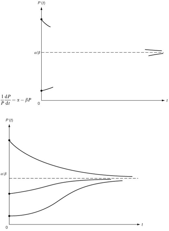
below the horizontal line P = α/β, our population will be increasing (α − β P > 0; so d P /d t > 0 until α − β P  0 near the line P = α/β and the curve will never actually cross this line.
In fact the exact solution of the differential equation
Figure 6.1
Figure 6.2