Data from the computer simulation are given in Table 9.15.

Figure 9.17 (see page 274) shows the path of the parachutist and Figure 9.18 (see page 275) shows how the speed varies with time.

9.9 On the buses

Context

Bus timetables are very difficult to put into reliable operation because of the many random and irregular factors which affect the running of the buses. Suppose that, as part of a study into the operation of driver-operated buses, you are asked to develop a model to look into the problem of ‘bunching’ of buses on the same regular route.

Problem statement

What should be the time interval between buses leaving the bus depot so that

1.buses on the route do not catch up with and/or overtake each other and

2.passengers do not have very long waits in between buses?

Figure 9.17

Formulate a mathematical model

This problem is clearly a candidate for the stochastic simulation treatment described in chapter 7. We

can develop, however, a simple deterministic model as a starting point, and the random elements can be introduced at a later stage. There are obviously three groups of factors involved: the buses, the bus stops and the passengers. So we can construct our factor list as follows.

Factors concerning the buses. Time of leaving the depot. Time of arrival at any stop.

Number of passengers leaving at any stop. Time spent at a stop.

Total number of passengers carried. Maximum capacity.

Speed of travelling. Traffic conditions.

Figure 9.18

Factors concerning the bus stops. Position of stop on the bus route. Time elapsed since the last bus left. Rate of arrival of passengers.

Number of passengers waiting when next bus arrives. Distance between stops.

Factors concerning the passengers. Time of arrival at a stop.

Length of journey (number of stops).

Waiting time for a bus. Total journey time.

There is obviously some overlap here and we need to construct a convenient notation so that we can express the connections between the factors and reduce the number of variables.

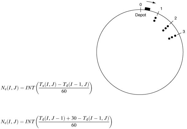
For simplicity, consider a circular route with stops at regular 0.25 mile intervals (Figure 9.19). If we ignore traffic delays and assume that the buses travel at a constant 30 miles h −1 , then all the journey times between stops will be 30 s. Assume that passengers arrive at any stop at an average rate of one per minute. The driver has to collect fares as passengers board his bus; assume that it takes a constant 10 s per passenger. Also assume that passengers take 5 s each to get off the bus and that the bus can carry up to a maximum of 60 passengers.

Suppose that a total number N b of buses leave the depot at regular intervals T with the first leaving at time 0 and the I th bus leaving at time ( I − 1) T. Let T a ( I, J ) be the time of arrival of bus I at stop J, T d ( I, J ) the time of departure of bus I from stop J, N 1 ( I, J ) the number of passengers leaving bus I at stop J and N e ( I, J ) the number of passengers entering bus I at stop J.

The time spent at stop J by bus I (which equals T d ( I, J ) − T a ( I, J )) is clearly determined by the maximum of {5 N 1 ( I, J ), 10 N e ( I, J )} . If we assume that the number of passengers waiting at stop J when bus I arrives is proportional to the time elapsed since the previous bus I − 1 left, we have

Figure 9.19 i.e.

for an arrival rate of one per minute where INT ( x ) stands for the integer part of x and is an alternative to the [] notation used in section 9.4. The first bus is rather special in this regard; so we can define T d (0, J ) = 0 for all J.

The number of passengers leaving bus I at stop J has to be worked out. We may have some data on the lengths of journeys made by passengers (Table 9.16).