3 APPENDICES

3.1Possible extensions

1.We have assumed that all the individuals tested have the same probability P of possessing the condition. If instead it is known that age or sex or some other easily identifiable factor affects an individual's probability of having the condition, then this could be taken into account when forming the groups. A more efficient procedure might then be possible.

2.We have described the testing procedures in terms of blood samples but the same conclusions could apply to more general situations. Suppose that some finite population is considered in which every item either does or does not possess a certain defect. We assume that from each item a product can be extracted (‘blood’) on which a test can be carried out which will reveal the presence of this defect. We wish to identify all the defective items using the minimum number of tests. If the test can be applied to pooled samples as effectively as to individual samples, then the conditions are equivalent to those considered in this report and the same conclusions will apply.

3.2Mathematical analysis

The graph of E(T)IN against K for the single-stage procedure corresponds to an equation of the form

where

To find the local extreme values of y, we differentiate with respect to K. This gives

which equals 0 when

Now, since x < 1, the expression K 2 x K considered as a function of K has a graph such as that sketched in Figure 2.

There is a local (and global) maximum for some value K = K * . We are looking for points where the graph is cut by the horizontal line at height − 1/In x. Clearly there will be no such points if − 1/In x >

m, where m is the maximum value of

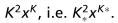
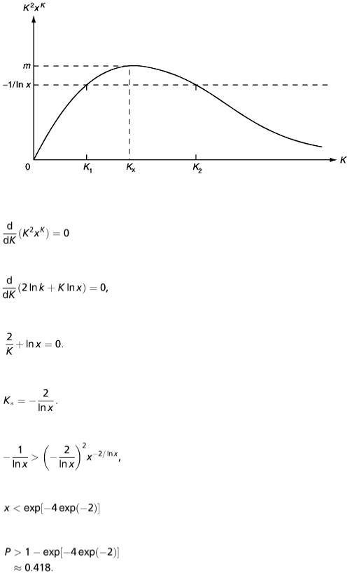
Figure 2

We find K * by solving

or

i.e.

Therefore,

There will be no roots if

i.e.

or