

2 MAIN SECTIONS
2.1 Problem statement
Suppose that we have a finite population of N individuals, each with a fixed probability of having a certain (rare) condition and we wish to identify all the affected individuals. We assume that samples of blood are available from all the individuals concerned and that a test is available which will detect the presence of the condition. If the testing procedure is expensive or difficult to carry out, we shall wish to minimise the total number of tests required to find all the affected individuals.
Suppose that it is possible to apply the test to the pooled blood sample from a number of individuals such that a positive result will be indicated if at least one of the individuals is affected. We can then save on the number of tests since a negative result will allow all individuals in the pool to be cleared.
There are a number of different testing procedures which could be used in these circumstances and the problem posed here is to find a procedure which will minimise the expectation of the total number of tests.
2.2 Assumptions
For the remainder of this report we shall assume the following.
1.The test in question can be applied to a pooled sample of blood made up from the samples taken from the individuals.
2.The test is 100% reliable in the sense that a negative response means that all individuals who contributed to the pooled sample must be clear and that a positive response will only be obtained when at least one individual in the pool is affected.
3.The amount of blood sampled from each individual is sufficient to be divided into a number of parts for subsequent testing.
4.Every individual involved has the same inherent probability P of being affected.
2.3Individual testing
The most direct procedure is of course to apply the test to every individual. We show in the next section that this is in fact the best procedure if P exceeds about 0.3 but for smaller values of P the use of pooled samples gives a saving in the expected number of tests.
2.4 Single-stage procedure
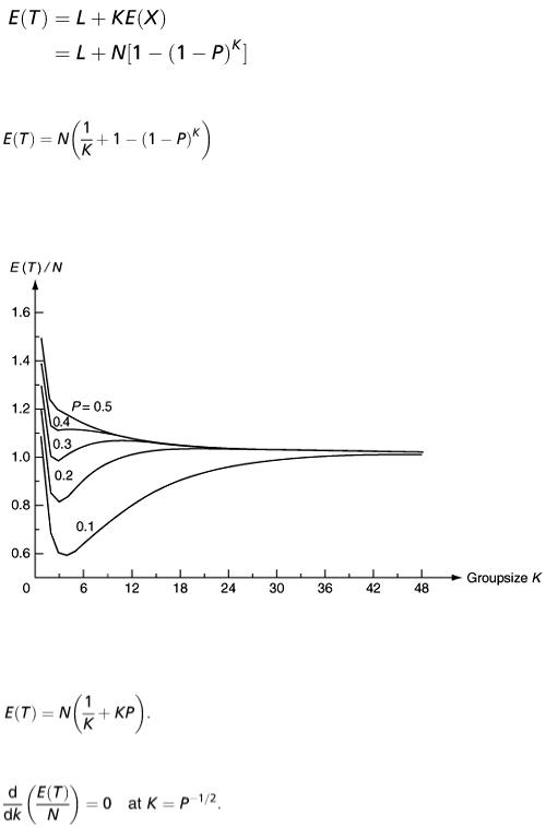
In this procedure, we divide the population into a number of groups ( L, say) and test a pooled sample from each group. Each group contains K = N/L individuals and each test is a Bernoulli trial with probability (1 − P ) K of a negative response. If X is the number of groups giving a positive response, the distribution of X will be binomial ( L, P ′), where P ′ = 1 − (1 − P ) K .
For each group with a positive response, all the individuals in that group will be tested. This requires XK tests. The expected number of tests is therefore
or, in terms of K, the size of each group,
(1)
K has to be an integer of course but, if we regard the expression on the right-hand side as a function of a continuous variable K, we obtain curves such as those shown in Figure 1. For values of P < 1 − exp[−4 exp (−4 exp (−2)](  0.418), the curves have a local minimum for K > 0 so that the expected number of tests can be minimised by an appropriate choice of K.
Figure 1
Equation (1) shows that the optimal choice of K depends on P only. We can get an approximation to this optimal K value for small P by using the relation 1 − (1 − P ) K  KP; then
Differentiation with respect to K gives
From the graphs in Figure 1 we see that, as K → ∞, we have 1/ K + 1 − (1 − P ) K → 1 so that E(T)/N can be brought close to 1 by choosing a sufficiently large value of K. In practice of course there is an upper limit on K given by the value of N . For values of P ≤ 1 − exp[− exp(−1)](  0.308), the local minimum for E(T)/N does give the overall minimum. For values of P larger than this, however, the overall minimum for E(T)/N is 1.0 and the best choice is to make K as large as possible, in other words to test each individual in the population.
The distribution of T/N can be found from the fact that T/N = 1/ K + KX / N where X is binomial
( N/K, 1 − (1 − P ) K ).
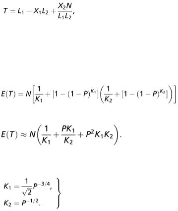
2.5 Two-stage procedure
In this procedure the first stage is to divide the population into L 1 groups with K 1 = N/L 1 individuals in each group and to test the pooled blood samples from each. This requires L 1 tests to be carried out. Suppose that X 1 of these are
positive. In the second stage, we divide all the positive groups into L 2 subgroups with K 2 = N/L 1 L 2 individuals in each and test the pooled blood samples from each subgroup. This requires X 1 L 2 tests. Suppose that X 2 of these tests are positive. For each positive result, we test every individual in that subgroup. The total number of tests for the whole procedure is
where the random variable X 1 has the binomial distribution ( L 1 , P ′) and the distribution of the random variable X 2 , conditional on X 1 , is binomial ( X 1 L 2 , P ′′), where P ′ = 1 − (1 − P ) N/L 1
and 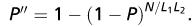 We have E ( X 1 ) = L 1 P ′ and E ( X 2 ) = L 1 L 2 P ′ P ′′, so that E(T) = L 1 + L 1 L 2 P ′ + NP ′ P ′′. As with the single-stage procedure, it is mathematically more convenient to express E (T) in terms of K 1 and K 2 , which give us
(2)
Using the approximation 1 − (1 − P ) X  XP for small P, we get
On setting the partial derivatives with respect to K 1 and K 2 equal to zero, we find that for a stationary point of E(T) regarded as a function of K 1 and K 2 we have
(3)
In actual fact, of course, K 1 / K 2 must be an integer. As with the single-stage procedure the optimal choices of K 1 and K 2 are independent of N, being dependent on P only.
2.6 Results
In Table 1 the values of K, K 1 and K 2 giving minimum E(T) are recorded for various values of P . These were found by direct search from the exact expressions (1) and (2). A marked reduction in the expected number of tests is revealed when the two-stage method is used, especially at low values of P. The approximations given in equations (3) are found to be reasonably accurate. For example, at P = 0.02, equations (3) give K 1 = 13 and K 2 = 7 while the actual optimum is at K 1 = 16, K 2 = 8. To indicate the distribution of T, a simulation was carried out using a random-number generator. The following results were obtained from 300 runs using a population size N = 96 (for convenience) and P = 0.02. The distribution of T using the two-stage procedure with K 1 = 16 and K 2 = 8 is as follows.
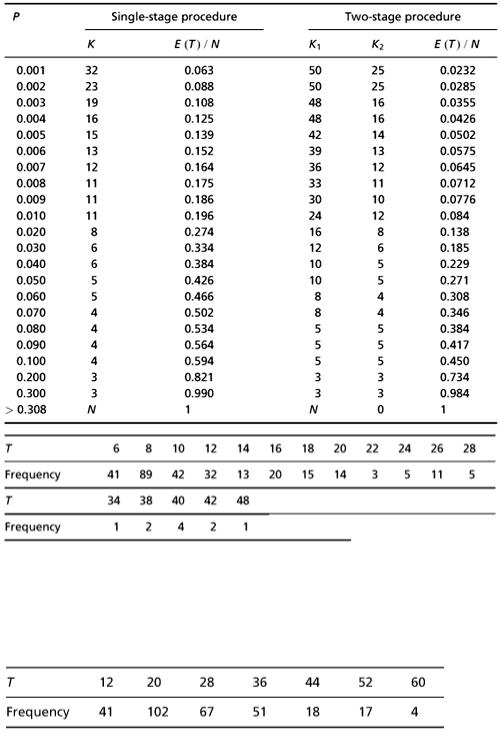
Table 1
This has a mean value  of 12.76 and a variance of 57.42. The calculated value of
  N is 0.133, which agrees well with the theoretical prediction of 0.138 from Table 1.
For comparison, a simulation of 300 runs using the single-stage procedure with K = 8 (for N = 96, P = 0.02) gave the following distribution of  .
.
This has a mean value  of 27.2 and a variance of 128.64. The calculated value of
  N is 0.283 compared with the theoretical value of 0.274.
2.7 Regular section procedures
In a bisection procedure an initial test of the pooled sample for the population, if proved positive, is