Football throw-in A throw-in is taken from a point roughly in line with the penalty spot with the intention of landing the ball on the ‘striker's’ head. The team coach has said that running up before throwing is necessary in order to make a long throw. Unfortunately there is a wind blowing directly across the field towards the thrower. Also a football is affected by air resistance, which is

6.10taken as directly proportional to the speed of the ball. Your job as modeller is to construct the equations of motion which define the path of the ball and to decide whether the striker is likely to have a chance of getting his head to the ball as it comes across. The data are as follows: the run-up speed of the thrower is 4 m s −1 , the speed of the throw (relative to the thrower) is 15 m s −1 , the wind velocity varies between 0 m s −1 and 15 m s −1 , and the air resistance constant (per unit mass) is 0.003 s −1 .

Basket shot When a foul occurs in a game of basketball, the attacking team may be awarded a free shot in which a player attempts, unhindered, to throw the ball into the basket from a certain position. In a way this is quite like the fireman problem, but the entry of the ball into the basket is now crucial since, as the thrower soon finds out, the ball is apt to strike the basket rim and to bounce out again! Obtain the two equations of motion again. Neglect air drag but this time the

6.11angle of flight of the ball is needed so that we can examine whether it will actually pass into the basket. Clearly the height of the thrower now matters and also the height of the gymnasium must place some restriction on the ball's trajectory. The data are as follows: the basketball diameter is 25 cm, the basket hoop diameter is 45 cm, the height of the gymnasium is 6.5 m, the distance of the throwing point from the basket is 4.6 m, and the height of the basket above the gymnasium floor is 3.05 m. Often a successful throw is achieved by rebound from the backboard, placed 0.5 m behind the centre of the basket rim. Can you incorporate this feature into your model?

Putting the shot In this problem, we wish to maximise the distance thrown by a shot putter, where the throw range is at a level different from the level of the throw projection point. The world record is currently around 23 m. The question for the mathematical modeller is to offer advice regarding the angle of throw. The projection speed remains about the same for all throws, the

6.12ambient conditions in a given competition can be discounted since shot putting is a fairly local activity, and so the variables reduce to the following.

1.The angle of throw.

2.The height of projection.

6.5 Simultaneous coupled differential equations

In many models the variables affect each other and the equation for the rate of change of one variable is very likely to involve the other variables as well. This leads to systems of coupled differential equations which as a rule are rather difficult to solve analytically. If time does not appear explicitly on the righthand side of our equations, we can simply divide one equation by another to obtain an equation not involving t. Suppose for example that we have the following equations:

Division gives

We could now go on to solve this differential equation, which would give us a set of curves in the x − y plane. This is sometimes called a ‘phase plot’. In this diagram, time does not appear explicitly but is implied in the sense that a particular curve in the phase plot shows how x and y change together as time passes. We can think of the state of our system as a moving point starting from a point determined by the initial values x (0), y (0), and subsequently moving along a solution curve of the differential equation, usually referred to as the ‘trajectory’. This can be very useful for determining the evolutionary behaviour of the model and for investigating how different starting values may lead to different final results.

What this diagram cannot do, however, is tell us how much time is required for the system to evolve from one point to another. To answer such questions, we have to go back to the original differential equations. We may be able to substitute for one variable from one equation into another and to solve the resulting differential equation. Alternatively, there are numerical techniques available for solving systems of coupled differential equations. If we use a numerical method, we also have to select starting values for our variables and usually the time step. We then obtain a print-out of the evolution of the model starting from the chosen initial conditions. To find out what happens from other starting conditions, we have to do separate runs of the model.

It is also worth considering what information we can get without solving the differential equations. In particular, it is often instructive to look at values of the variables (if any) which make the derivatives equal to zero. These are known as the ‘equilibrium points’ and they can have any of a number of

different stability properties. We can also look for restrictions on the values of the variables implied by the signs of the derivatives.

Example 6.5 Modelling a battle Context

The X army is about to attack the Y army which has only 5000 troops while the X army has 10 000. The Y army, however, has superior military equipment which makes each Y soldier 1.5 times as effective as an X soldier.

Objective

We wish to develop a mathematical model for the resulting battle and use the model for the following purposes.

1.To predict which army will win.

2.To estimate how many troops of the winning army will be left at the end.

3.To calculate how many troops the losing army would have needed initially in order to win the battle.

Formulate a mathematical model

Before getting around to developing a model for this specific problem, let us look at the assumptions we can reasonably make when modelling a battle between two opposing forces. Our variables are x ( t ), the number of X troops alive at time t, and y ( t ), the number of Y troops alive at time t. As in

(6.19)

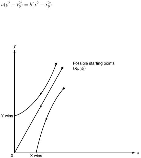
In the x − y plane the solution curve is part of a hyperbola as shown in Figure 6.15.

Suppose, as a special case, that the initial sizes of the two armies are such that then equation (6.19) reduces to ay 2 = bx 2 or This means that the solution curve is the straight line through the origin with slope and the battle progresses inexorably from the point

Figure 6.15

( x 0 , y 0 ) to the point (0, 0). We conclude from this that the condition for an evenly matched battle (one that results in mutually assured destruction) is .

It follows that a sensible measure of any army's fighting strength can be obtained from the square of its size multiplied by its kill rate. This was pointed out by Lanchester in 1914 and is known as Lanchester's square law.

If then the point ( x 0 , y 0 ) is above the straight line of equal fighting strengths in Figure 6.15 and the Y army will win. We can also check this from the general solution (6.19).

For the X army to win, we would have to have y = 0 while x is still greater than zero, and from equation (6.19) we would then have 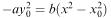so that 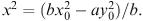However, we have assumed that ; so this equation has no solution in real numbers. On the other hand, equation

(6.19) predicts that x = 0 when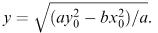

According to our assumption that the initial values satisfy this gives a meaningful value for y which is in fact our model's prediction for the number of survivors of the Y army at their moment of victory.

Returning to our initial example, let us choose an hour as our unit of time and assume that 0.15 X soldiers are killed by each Y soldier in 1 h and that 0.1 Y soldiers are killed by each X soldier in 1 h. Our difference equations are x = −0.15 y t and y = −0.1 x t, where t = 1 h. We shall get approximately the same solutions if we solve the differential equations.

Our starting values are x 0 = 10 000 and y 0 = 5000. The fighting strength of the X army is 0.1 × (10 000) 2 = 10 × 10 6 while the fighting strength of Y is 0.15 × (5000) 2 = 3.75 × 10 6 . Our model

With the original values of x 0 = 10 000 and y 0 = 5000, how long will the battle last? This is not so easy to answer but we can get estimates without actually solving the equations.

Initially, we have 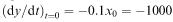; so at the start of the battle the Y troops are being killed at the rate of 1000 per hour. If this rate continued (in reality, it will not because the X army is also being reduced) the Y army would be totally wiped out in 5000/1000 = 5h. The battle must therefore last at least 5h. We can also find an upper bound for the duration of the battle by considering the rate at which the Y troops are being killed towards the end of the battle. We know from our calculations that there

will be about 7906 X troops alive at that time; so . If this had the same constant value from the beginning of the battle, then we would have the simple model y = −790.6 t + 5000 which predicts y = 0 at t = 5000/7906 6.32.

We now know that the battle will last between 5 h and 6.32 h and a midpoint estimate would be 5.7 h. These thoughts are illustrated in Figure 6.16. The exact answer can be found by solving the differential equations. Differentiating the first equation, we have

and substituting for d y /d t from the second equation, this becomes

or

This has a solution of the form

(6.20)

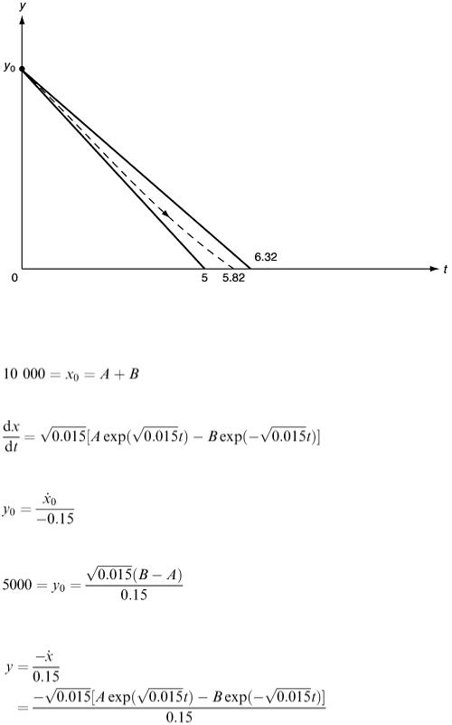
Figure 6.16

where the constants A and B can be found from the facts that x 0 = 10 000 and y 0 = 5000. Substituting t = 0, we have

(6.21)

The second fact is less easy to use. If we differentiate equation (6.20), we get

and we know that

So

(6.22)

Solving equations (6.21) and (6.22) for A and B, we get A 1938.14 and B 8061.86. The size of the Y army at any time is

From this we deduce that y = 0 when 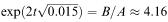, which gives t 5.82 h, confirming our previous estimate.

We calculated earlier that, for the Y army to win the battle, they would have needed 3165 extra troops at the beginning. Suppose reinforcements for the Y army become instantly available (e.g. paratroops) at

some time after the beginning of the battle. We can calculate the number N needed for Y to go on to win the battle from the fact that we need at least to make up the difference in fighting strength at that moment, i.e.

This gives the following results.

Note that equations (6.17) and (6.18) constitute a simple battle model. Many other (and better) models are possible using different differential equations based on more careful assumptions.

Example 6.6 Foxes and rabbits Context

Suppose that some rabbits and foxes are living in a confined area where there is plenty of food for the rabbits and the foxes depend on eating rabbits for their food.

Objective

Develop a model that will enable us to predict the numbers of rabbits and foxes alive at any time t. Formulate a mathematical model

Our variables are x, the number of rabbits at time t and y, the number of foxes at time t. To proceed with the model we need some assumptions. Suppose that left to themselves, i.e. in the absence of foxes, the rabbits would increase their numbers by a factor of about 4 in one time unit. We can model the growth of the rabbits by the differential equation

Note that the exact solution of this is x(t) = x (0)e 1.4 t which is an example of exponential growth and in one time unit the rabbit population is multiplied by the factor e 1.4 which is about 4.0552. If there were no rabbits the foxes would starve to death. Suppose this would be at a rate of about 90% per time unit. This means that (approximately)

When both rabbits and foxes exist together, it is reasonable to assume that the rate at which rabbits are killed by foxes is proportional to the number of rabbits and also proportional to the number of foxes. Also the more food there is for them the healthier the foxes become and the more young foxes are born. With these interactions included our differential equation for the rabbits takes the form

The constant 0.02 represents the proportion of the rabbit population killed by one fox in one time unit. (The value 0.02 is an arbitrary choice in the absence of real data.) Similarly our differential equation for the foxes becomes extended to

Here the constant 0.001 represents the proportion of extra births in the fox population per time unit due to the food value of one rabbit (again an arbitrary numerical choice).

Comparing the two differential equations that we have just written down with equations (6.17) and (6.18), we see similarities and differences. The xy terms on the right-hand sides of the equations, representing the interaction between the two populations, are present this time but with a positive sign in the case of the foxes. Also both equations have a linear term representing a natural birth rate in the case of the rabbits and a natural death rate in the case of the foxes. To investigate equilibrium points we set d x /d t = 0 = d y /d t , i.e.

One solution is obviously x = 0, y = 0, when there is no life at all. Another is given by solving 1.4 – 0.02 y = 0 and 0.001 x − 0.1 = 0, which gives x = 100 and y = 70. According to this model and under these conditions, 100 rabbits and 70 foxes would live ‘harmoniously’ together and their numbers would remain at these levels indefinitely.

If we try the values x (0) = 100 and y (0) = 40, we find a cyclic behaviour in both rabbit and fox populations, as shown in Figure 6.17.

Figure 6.17

The rabbit population oscillates between about 6 and about 430, the whole cycle repeating itself with a period of about 19.6 time units.

The oscillation in the fox population is from 40 to about 112 with the same period.

In the phase diagram (Figure 6.18), we see the rabbit and fox population levels plotted one against the other and the trajectory is a closed curve, which is traversed once every 19.6 time units approximately. The initial point is marked P and the arrows show the direction in which the trajectory is traversed. The

point E is the equilibrium point (100, 70).

At points along the section of the curve marked A, both populations are increasing. Note that in this region we have x > 100 and y < 70 and the differential equations give d x /d t > 0 and d y /d t > 0, confirming what we have just said. In the section marked B, having crossed the horizontal line where y = 70, we have d x /d t < 0, while d y /d t > 0. Our interpretation of this is that there are now so many foxes that the rabbit population is decreasing. In section C there is not enough food for the foxes and so they decrease as well as the rabbits ( x < 100 and y > 70 and so d x /d t < 0 and d y /d t < 0).

Along section D, there are so few foxes that the rabbits are able to begin to increase their numbers again and we return to point P. Note that the maximum and minimum values of y occur when x = 100, the equilibrium value, and d y /d x = 0, while the maximum and minimum values of x occur when y = 70, the equilibrium value, and d y /d x = ∞. We cannot find the actual maximum and minimum values, however, without solving the differential equations.

If we start with different values of x (0) and y (0), we find a similar behaviour with a trajectory in the form of another closed curve going round the equilibrium point.

Figure 6.18

However, if we make things very unfavourable for the rabbits by lowering their birth rate and revising upwards our estimate of the effect of the foxes on the rabbit population, so that the differential equation for the rabbits reads something like

With the other differential equation unchanged, and starting with 100 rabbits and 100 foxes, we find that after 4.6 time units we are down to fewer than one rabbit and about 68 foxes. If, regardless of this disaster for the rabbits, we continue with our model, we find that the rabbit population reaches a minimum of about 0.13 after 11.4 time units and then recovers, while the fox population reaches a minimum of 7.02 after 29.2 time units, after which time both populations are increasing together.

We now realise that for the sake of realism we should have stated at the outset that our model applies

only when x > 1 and y > 1. The conclusion from our last run of the model is that the rabbits would all have been wiped out after about 4.6 time units and the foxes would then either have to find an alternative food supply or die themselves.

You will recall that we chose the coefficients in the differential equations arbitrarily and Figures 6.17 and 6.18 show the results. Curves similar to these have in fact been obtained from real data. An example is the interaction between the Canadian lynx and hare.

Example 6.7

In chapter 5 there was Example 5.5 involving two lakes. The details are on Figure 5.5 which we modelled as a discrete system. Let us now reconsider this example as a continuous system. Let c denote the volume fraction of pollution ( c will be a number between 0 and 1). This means that every m 3 of lake water contains c m 3 of pollution. Using c 1 and c 2 for the first and second lakes, the total amount (m 3 ) of pollution in the two lakes is 100 000 c 1 and 50 000 c 2 respectively and their rates of change are 100 000 c ′ 1 and 50 000 c ′ 2 . The rate of input of pollution to the first lake is 5 (m 3 d −1 ) and every day 1000 m 3 of polluted water flows out of this lake (each m 3 containing c 1 m 3 of pollution). The rate of output of pollution from lake 1 is therefore 1000 c 1 and we can write down a differential equation for lake 1:

The output from lake 1 becomes the input to lake 2 so the equation for lake 2 is:

To solve the problem we need initial values c 1 (0) and c 2 (0), suppose for the moment that initially these are both zero. With time they will both clearly increase and to find the time behaviour exactly we need to solve the differential equations with these starting values. However, we can make some predictions from the equations without solving them. Note that c ′ 1 will approach zero as c 1 approaches 0.005. In other words as it approaches 0.005, c 1 will stop changing and can never grow

beyond that level. With c 1 at this level the equation for c 2 will become from which we see that c 2 will also stop changing when it reaches 0.004167. Figure 6.19 shows graphs obtained by solving the differential equations for c 1 and c 2 confirming these predictions.

Figure 6.19

Exercises

6.13 In the above battle model, if the Y army had the minimum necessary number of troops to win, how

long would the battle last?

6.14If instead of entering the battle en masse at a particular moment, the reinforcements arrived at a continuous constant rate, how would you modify the model?

Two different species of insect live together and eat the same food. They do not interfere with each other apart from the fact that they are competing for food. Make the following assumptions.

Derive a mathematical model based on these assumptions and use it to investigate what happens to the two populations for various initial values and using different values of the coefficients in the differential equations.

6.16In the ‘rabbits and foxes’ model

1.What is the period (time it takes to go round the loop once)?

2.Note that the peak in the fox population lags behind the peak in the rabbit population. What is the lag?

3.Find what happens when different values are put in for the coefficients in the differential equations.

4.We assumed a constant proportion of the rabbit population is killed by each fox in one time unit. Would it be more realistic to assume a constant number of rabbits killed by each fox, in which case how would you modify the equations?

5.Can you extend the model to include grass? You will need to make assumptions about the rate of growth of grass with time and the rate at which it is eaten by the rabbits.

6.Suppose foxes or rabbits or both are also killed by humans. How do you incorporate these